CS Concepts

本章笔记着重对CS相关专业科目的名词进行解释，在修考问答题和面试八股文场景下适用。这些名词都来源于CS相关学科。本篇笔记内容按科目划分，每个科目下面有对应的常见高频名词解释（中/英）。

1. Data Stucture & Algorithms

Hash Table

A Hash Table is a data structure that maps keys to values using a hash function. It stores data in an array-like structure, where each key is hashed to an index. Collisions (when different keys map to the same index) are handled using techniques like chaining or open addressing. Hash tables provide average O(1) time complexity for insertion, deletion, and lookup. They are widely used in databases, caching, and symbol tables.

Hash Collision / Hash Clash

A hash collision (hash clash) occurs when two different inputs produce the same hash value in a hash function. Since hash functions map a large input space to a smaller output space, collisions are inevitable due to the pigeonhole principle. Collisions can weaken security in cryptographic hashes (e.g., MD5, SHA-1) and reduce efficiency in hash tables. Techniques like chaining, open addressing, and better hash functions help mitigate collisions. Stronger cryptographic hashes (e.g., SHA-256) minimize the risk of intentional hash clashes (collision attacks).

Open Addressing / Closed Hashing

Open addressing is a collision resolution technique in hash tables where all elements are stored directly in the table without external chaining. When a collision occurs, the algorithm searches for the next available slot using a probing sequence (e.g., linear probing, quadratic probing, or double hashing). Linear probing checks the next slot sequentially, quadratic probing uses a quadratic function to find slots, and double hashing applies a second hash function for probing. Open addressing avoids linked lists, reducing memory overhead but may suffer from clustering. It works best when the load factor is kept low to maintain efficient lookups.

Seperate Chaining

Separate chaining is a collision resolution technique in hash tables where each bucket stores multiple values using a linked list (or another data structure like a BST). When a collision occurs, the new element is simply added to the linked list at that index. This method allows the table to handle an unlimited number of collisions but increases memory usage. Performance depends on the length of the chains; with a well-distributed hash function, the average lookup time remains O(1) in best case and O(n) in worst case. Rehashing or using a larger table can help maintain efficiency.

P ≠ NP

P ≠ NP means that not all problems whose solutions can be verified quickly (in polynomial time) can also be solved quickly.
P is the class of problems that can be solved in polynomial time.
NP is the class of problems whose solutions can be verified in polynomial time.
The question is: if a problem’s solution can be verified quickly, can it also be found quickly?
Most experts believe P ≠ NP, but it has not been proven yet.

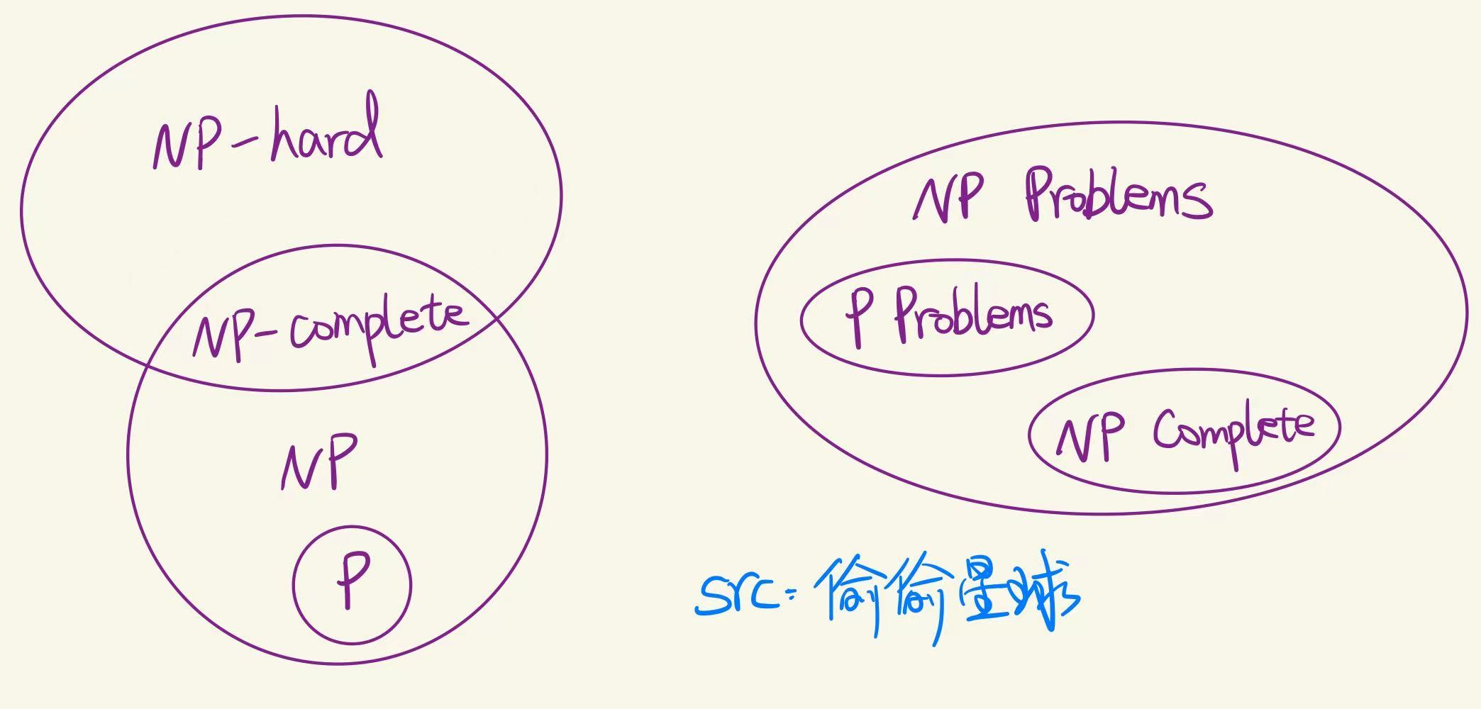
NP Hard Problems

NP-Hard problems are computational problems that are at least as difficult as the hardest problems in NP (nondeterministic polynomial time). Solving an NP-Hard problem quickly would mean we could solve every NP problem quickly too, but no such efficient solution is known. These problems may not even have verifiable solutions in polynomial time. They often involve optimization or decision-making with many possibilities, like scheduling, routing, or packing.Examples include the Traveling Salesman Problem and Knapsack Problem.

NP-Complete Problems

NP-Complete problems are a special class of problems that are both:

In NP – their solutions can be verified in polynomial time, and
NP-Hard – as hard as the hardest problems in NP.

If you can solve any NP-Complete problem quickly (in polynomial time), you can solve all NP problems quickly. Famous examples include the Boolean Satisfiability Problem (SAT) and Traveling Salesman Problem (decision version).

The Travelling Salesman Problem

The Travelling Salesman Problem (TSP) asks for the shortest possible route that visits each city once and returns to the starting city.
It is a classic combinatorial optimization problem in computer science and operations research.
TSP is NP-hard, meaning there’s no known efficient algorithm to solve all cases quickly.
Exact solutions use methods like brute force, dynamic programming, or branch and bound.
Approximation and heuristic algorithms (e.g. genetic algorithms, simulated annealing) are used for large instances.

The Knapsack Problem

The Knapsack Problem asks how to choose items with given weights and values to maximize total value without exceeding a weight limit.
Each item can be either included or excluded (0-1 Knapsack).
It’s a classic NP-hard optimization problem.
Dynamic programming is commonly used for exact solutions.
Greedy or approximation methods are used for large instances.

The SAT (Boolean Satisfiability) problem

The SAT (Boolean Satisfiability) problem asks whether there exists an assignment of true/false values to variables that makes a Boolean formula true.
It’s the first problem proven to be NP-complete.
The formula is usually given in CNF (Conjunctive Normal Form).
SAT solvers use techniques like backtracking and clause learning.
Many real-world problems (e.g. planning, verification) can be reduced to SAT.

Divide and Conquer

Divide and Conquer is a problem-solving strategy that works in three main steps:

Divide the problem into smaller sub-problems of the same type.
Conquer each sub-problem by solving them recursively.
Combine the solutions of sub-problems to get the final result.

Classic examples include Merge Sort, Quick Sort, and Binary Search.

Branch and Bound

Branch and Bound is an algorithmic paradigm for solving combinatorial optimization problems efficiently. It systematically divides the solution space into smaller subproblems (branching) and computes bounds to eliminate unpromising branches early (pruning). The method maintains an upper bound from feasible solutions and a lower bound from relaxed problems, allowing it to discard branches that cannot contain the optimal solution. This approach significantly reduces the search space compared to exhaustive enumeration, making it effective for problems like integer programming, traveling salesman, and knapsack problems.

B-tree

A B-tree is a self-balancing search tree that maintains sorted data for efficient insertion, deletion, and search in O(log n) time.
It allows each node to have multiple keys and children, making it wider and shallower than binary trees.
All leaf nodes are at the same level, ensuring the tree stays balanced.
It’s widely used in databases and file systems for fast disk-based access.

Heap Sort

Heap Sort is a comparison-based sorting algorithm that uses a binary heap data structure. It works in two main steps:

Build a Max Heap from the input data so that the largest element is at the root.
Extract the root (maximum element), swap it with the last item, reduce the heap size, and heapify the root to maintain the max heap. Repeat until the heap is empty.

Time Complexity: Best, Average, Worst: O(n log n)

Key Characteristics:

In-place sorting (no extra space needed)
Not stable
Good for scenarios where memory is limited and performance is important.

Merge Sort

Merge Sort is a divide and conquer sorting algorithm that divides the input array into smaller parts, sorts them, and then merges the sorted parts.

Steps:

Divide the array into two halves.
Recursively sort each half.
Merge the two sorted halves into one sorted array.

Time Complexity:

Best, Average, Worst: O(n log n)

Key Characteristics:

Stable sort
Not in-place (uses extra space for merging)
Great for sorting linked lists or large datasets with consistent performance.

Quick Sort

Quick Sort is a divide and conquer sorting algorithm that works by selecting a pivot element and partitioning the array into two parts:

Steps:

Choose a pivot (e.g., first, last, or random element).
Partition the array: elements less than pivot go left, greater go right.
Recursively apply Quick Sort to the left and right parts.

Time Complexity:

Best & Average: O(n log n)
Worst (unbalanced partition): O(n²)

Key Characteristics:

In-place
Not stable
Very fast in practice with good pivot selection

A* Algorithm

The A* algorithm finds the shortest path by combining actual cost from the start (g) and estimated cost to the goal (h).
It selects nodes with the lowest total cost f(n) = g(n) + h(n).
It uses a priority queue to explore the most promising paths first.
The heuristic h(n) must not overestimate to ensure optimality.
It’s widely used in games, maps, and AI for efficient pathfinding.

Minimax Algorithm

The Minimax algorithm is used in two-player games to find the optimal move by assuming both players play optimally.
It recursively explores all possible moves, maximizing the player’s score and minimizing the opponent’s.
“Max” tries to get the highest score; “Min” tries to get the lowest.
The game tree is evaluated using a scoring function at terminal states.
It’s often optimized with alpha-beta pruning to skip unnecessary branches.

🤖 Alpha-Beta Pruning

Alpha-Beta Pruning is an optimization technique for the Minimax algorithm used in two-player games (like chess or tic-tac-toe).
It reduces the number of nodes evaluated in the game tree without affecting the final result.

🧠 How It Works

Alpha (α): the best already explored value for the maximizing player.
Beta (β): the best already explored value for the minimizing player.

While traversing the tree:

If the current branch cannot possibly influence the final decision (because it’s worse than previously examined branches), it is pruned (skipped).

✅ Benefits

Same result as Minimax, but faster
Reduces time complexity from O(b^d) to O(b^(d/2)) in the best case
(where b is branching factor, d is depth)

📌 Example

In a minimax tree:

If a max node finds a value ≥ β, it stops exploring further children.
If a min node finds a value ≤ α, it prunes the remaining branches.

🎯 Use Cases

AI game engines
Decision-making in adversarial environments
Game tree search optimization

2. Operating System

Procss & Thread

A process is the basic unit of resource allocation and scheduling in an operating system, with its own independent address space and resources. A thread is the basic unit of CPU scheduling, and a process can contain multiple threads that share the process’s memory and resources. Threads switch faster and have lower overhead, making them suitable for concurrent execution. In contrast, processes are independent of each other, with higher switching overhead but greater stability. While multithreading improves execution efficiency, it also introduces challenges such as synchronization and mutual exclusion.

Semaphore

A semaphore in an operating system is a synchronization tool used to manage concurrent access to shared resources by multiple processes or threads.

Key Points:

It is an integer variable that controls access based on its value.
There are two main operations:
- wait (P): Decreases the semaphore value. If the result is negative, the process is blocked.
- signal (V): Increases the semaphore value. If there are blocked processes, one is unblocked.

Types:

Binary Semaphore: Takes values 0 or 1, similar to a mutex.
Counting Semaphore: Can take non-negative integer values, used to control access to a resource with multiple instances.

Use Case:

Semaphores help avoid race conditions, deadlocks, and ensure mutual exclusion in critical sections.

Example use: Controlling access to a printer shared by multiple processes.

Critical Section

A Critical Section in an operating system is a part of a program where a shared resource (like a variable, file, or device) is accessed. Since shared resources can be corrupted if accessed by multiple processes or threads simultaneously, only one process should enter the critical section at a time.

Key Concepts:

Mutual Exclusion: Ensures that only one process is in the critical section at any given time.
Entry Section: Code that requests entry to the critical section.
Exit Section: Code that signals the process is leaving the critical section.
Remainder Section: All other code outside the critical section.

Goals of Critical Section Management:

Mutual Exclusion – Only one process in the critical section at a time.
Progress – If no process is in the critical section, one of the waiting processes should be allowed to enter.
Bounded Waiting – A process should not wait forever to enter the critical section.

Tools Used:

Semaphores
Mutexes
Monitors
Locks

These tools help implement and manage access to critical sections safely.

3. Computer Architecture

Pipeline hazard

A pipeline hazard in computer architecture refers to a situation that prevents the next instruction in the pipeline from executing at its expected time, causing delays.

Types of Pipeline Hazards:

Data Hazard:
Occurs when instructions depend on the result of a previous instruction that hasn’t completed yet.
Example:
```
ADD R1, R2, R3  
SUB R4, R1, R5  ← depends on R1
```
Control Hazard (Branch Hazard):
Happens when the pipeline makes wrong predictions about instruction flow, such as branches or jumps.
Structural Hazard:
Arises when hardware resources are insufficient to support all instructions in parallel (e.g., one memory unit shared by two stages).

Solution Techniques:

Forwarding (data hazard)
Stalling (inserting bubbles)
Branch prediction (control hazard)
Adding hardware units (structural hazard)

Pipeline hazards reduce performance and must be carefully handled in modern CPUs.

Data hazard

A data hazard occurs in a pipelined processor when an instruction depends on the result of a previous instruction that has not yet completed, causing a conflict in data access.

Types of Data Hazards:

RAW (Read After Write) – Most common
An instruction needs to read a register that a previous instruction will write, but the write hasn’t happened yet.
Example:
```
ADD R1, R2, R3  
SUB R4, R1, R5  ← needs R1 before it's written
```
WAR (Write After Read) – Rare in simple pipelines
A later instruction writes to a register before an earlier instruction reads it.
WAW (Write After Write) – Happens in out-of-order execution
Two instructions write to the same register in the wrong order.

Solutions:

Forwarding (bypassing) – Pass result directly to the next instruction.
Stalling – Delay the dependent instruction until data is ready.

Data hazards can slow down pipeline performance if not properly managed.

Control hazard

A control hazard (also called a branch hazard) occurs in pipelined processors when the flow of instruction execution changes, typically due to branch or jump instructions.

Cause:

The processor doesn’t know early enough whether a branch will be taken, so it may fetch the wrong instructions.

Example:

BEQ R1, R2, LABEL   ; Branch if R1 == R2
ADD R3, R4, R5      ; May be wrongly fetched if branch is taken

Solutions:

Branch Prediction – Guess whether the branch will be taken.
Branch Delay Slot – Always execute the instruction after the branch.
Pipeline Flushing – Discard wrongly fetched instructions.
Early Branch Resolution – Move branch decision to earlier pipeline stage.

Control hazards can reduce pipeline efficiency by introducing stalls or flushes.

Structural hazard

A structural hazard occurs in a pipelined processor when two or more instructions compete for the same hardware resource at the same time, and the hardware cannot handle all of them simultaneously.

Example:

If the CPU has one memory unit shared for both instruction fetch and data access, a conflict arises when:

One instruction is being fetched, and
Another instruction needs to read/write data from memory at the same time.

Solution:

Add more hardware resources (e.g. separate instruction and data memory – like in Harvard architecture)
Stall one of the instructions to resolve the conflict

Structural hazards are less common in modern CPUs due to better hardware design but can still occur in resource-limited systems.

Dynamic Branch Prediction

Dynamic Branch Prediction is a technique used in modern CPUs to predict the outcome of branch instructions (e.g., if-else, loops) at runtime, based on the history of previous executions.

Key Features:

Learns from past behavior of branches.
Updates prediction as the program runs.
More accurate than static prediction (which always predicts taken/not taken).

Common Methods:

1-bit predictor:
Remembers the last outcome (taken or not taken).
2-bit predictor:
More stable; uses a state machine to change prediction only after two mispredictions.
Branch History Table (BHT):
Stores past branch outcomes and uses them for prediction.
Global History & Pattern History Table (PHT):
Tracks patterns of multiple branches for more accuracy (used in two-level predictors).

Benefit:

Improves pipeline efficiency by reducing control hazards and minimizing stall cycles caused by branch mispredictions.

–

Instruction-level Parallelsim

Instruction-Level Parallelism (ILP) refers to the ability of a CPU to execute multiple instructions simultaneously during a single clock cycle.

Key Idea:

Many instructions in a program are independent and can be executed in parallel, rather than strictly one after another.

Types of ILP:

Compiler-Level ILP (Static ILP)
The compiler rearranges instructions at compile time to exploit parallelism (e.g., instruction scheduling).
Hardware-Level ILP (Dynamic ILP)
The CPU detects parallelism at runtime, using features like:
- Pipelining
- Superscalar execution (multiple execution units)
- Out-of-order execution
- Speculative execution

Example:

ADD R1, R2, R3  
MUL R4, R5, R6   ; Independent → can run in parallel with ADD

Benefits:

Increases CPU performance without increasing clock speed
Makes better use of CPU resources

Limitations:

Data, control, and structural hazards limit ILP
Dependence between instructions reduces parallelism

Modern processors heavily rely on ILP for high-speed performance.

Clock frequency

Clock frequency (also called clock speed) is the rate at which a processor executes instructions, measured in Hertz (Hz) — typically in gigahertz (GHz) for modern CPUs.

Key Points:

1 GHz = 1 billion cycles per second
Each clock cycle is a tick of the CPU’s internal clock, during which it can perform basic operations (like fetch, decode, execute).
A higher clock frequency generally means the CPU can perform more operations per second.

Example: A CPU with 3.0 GHz can perform 3 billion clock cycles per second.

Higher clock speed doesn’t always mean better performance, because:

Other factors like Instruction-Level Parallelism (ILP), number of cores, cache, and architecture efficiency also matter.
Very high clock speeds can cause more heat and power consumption.

Clock frequency = speed of instruction processing, but not the only factor in CPU performance.

Register renaming

Register renaming is a technique used in modern CPUs to eliminate false data dependencies (also called name dependencies) between instructions, allowing for more instruction-level parallelism (ILP) and better performance.

Why It’s Needed?

In pipelined or out-of-order execution, instructions may appear dependent due to using the same register name, even when there’s no real data dependency.

There are two main false dependencies:

Write After Write (WAW)
Write After Read (WAR)

Example (with false dependency):

1. ADD R1, R2, R3  
2. SUB R1, R4, R5  ← falsely depends on instruction 1 (WAW)

Both write to R1, but they’re unrelated operations. Register renaming removes this conflict.

How It Works:

The CPU maintains a larger set of physical registers than the number of logical (visible) registers.
It dynamically assigns different physical registers to each instruction, even if they use the same logical name.
This avoids name-based conflicts, enabling out-of-order and parallel execution.

Benefits:

Eliminates false dependencies
Increases parallelism
Improves CPU throughput

Summary:

Register renaming helps CPUs run more instructions in parallel by resolving unnecessary register name conflicts, boosting performance.

Sign-Magnitude Representation (原码)

Sign-Magnitude Representation (原码) is a binary method for representing signed integers.

Sign bit: The most significant bit indicates the sign — 0 for positive, 1 for negative.
Magnitude bits: The remaining bits represent the absolute value of the number in binary.

Example (using 8 bits):

+5 in sign-magnitude: 00000101
-5 in sign-magnitude: 10000101

Features:

Symmetrical representation for positive and negative numbers
Has two representations of zero: 00000000 (+0) and 10000000 (−0)

Since arithmetic operations with sign-magnitude require handling the sign separately, it is less efficient in hardware compared to two’s complement.

One’s Complement (反码)

One’s Complement (反码) is a binary method for representing signed integers.

Positive numbers: Same as in regular binary.
Negative numbers: Invert all bits of the positive number (i.e., change 0 to 1 and 1 to 0).

Example (using 8 bits):

+5: 00000101
-5: 11111010 (one’s complement of 00000101)

Features:

Two representations of zero: 00000000 (+0) and 11111111 (−0)
Subtraction can be done using addition, but still needs end-around carry handling.

Less efficient than two’s complement for arithmetic operations.

Two’s Complement (补码)

Two’s Complement (补码) is the most common binary method for representing signed integers.

Positive numbers: Same as regular binary.
Negative numbers: Invert all bits of the positive number (get the one’s complement), then add 1.

Example (using 8 bits):

+5: 00000101
-5: 11111011 (one’s complement of 00000101 is 11111010, plus 1 gives 11111011)

Features:

Only one zero: 00000000
Arithmetic operations (addition and subtraction) are simple and efficient
Widely used in modern computers for signed integer representation

Benchmark

Benchmark refers to a standardized test or reference used to evaluate the performance or quality of a system, device, program, or product.

A benchmark is a method of assessing the performance of an object by running a set of standard tests and comparing the results to others. It helps measure efficiency and identify areas for improvement.

Common Use Cases

Computer Hardware:
- Benchmarking CPUs, GPUs, SSDs, etc., by running performance tests and comparing scores.
- Common tools: Cinebench, Geekbench, PCMark.
Software Development:
- Measuring the speed or efficiency of code or algorithms to optimize performance.
Business Management:
- Comparing business performance to industry best practices to find room for improvement.

Big-endian

Big-endian is a type of byte order where the most significant byte (MSB) is stored at the lowest memory address, and the least significant byte is stored at the highest address.

Suppose we have a 32-bit hexadecimal number: 0x12345678

In Big-endian format, it would be stored in memory like this (from low to high address):

Address	Byte Value
0x00	0x12
0x01	0x34
0x02	0x56
0x03	0x78

Characteristics:

Commonly used in network protocols (e.g., TCP/IP), hence also known as network byte order.
The opposite of Big-endian is Little-endian, where the least significant byte comes first.

Little-endian (Brief Explanation)

Little-endian is a type of byte order where the least significant byte (LSB) is stored at the lowest memory address, and the most significant byte is stored at the highest address.

Suppose we have a 32-bit hexadecimal number: 0x12345678

In Little-endian format, it would be stored in memory like this (from low to high address):

Address	Byte Value
0x00	0x78
0x01	0x56
0x02	0x34
0x03	0x12

Characteristics:

Commonly used in x86 architecture (Intel and AMD CPUs).
It is the opposite of Big-endian, which stores the most significant byte first.
Easier for some CPUs to handle arithmetic operations on varying byte lengths.

Temporal Locality (时间局部性)

Temporal locality is a common program behavior in computer systems that means:

“If a data item is accessed, it is likely to be accessed again in the near future.”

Consider the following code snippet:

for (int i = 0; i < 100; i++) {
    sum += array[i];
}

When array[0] is accessed, the program will soon access array[1], array[2], etc.
The variable sum is also accessed repeatedly.
This demonstrates temporal locality.

Additional Notes:

Caches take advantage of temporal locality to improve performance.
Temporal locality commonly appears in:
- Loop variables
- Frequently called functions
- Intermediate computation results

Spatial Locality (空间局部性)

Spatial locality is a common program behavior in computer systems that means:

“If a data item is accessed, nearby data items (in memory) are likely to be accessed soon.”

Consider the following code snippet:

for (int i = 0; i < 100; i++) {
    sum += array[i];
}

When array[0] is accessed, the program will likely access array[1], array[2], …, array[99] shortly after.
These elements are stored in adjacent memory locations, so this illustrates spatial locality.

Additional Notes:

Caches use spatial locality by loading not just a single data item but also nearby memory blocks (called a cache line).
Spatial locality commonly appears in:
- Sequential array access
- Traversal of linked lists or other data structures with contiguous memory
- Instruction fetches during linear code execution

Hardware Prefetching (a.k.a. Prefetch)

Hardware Prefetching is a technique where the CPU automatically predicts and loads data into the cache before it is actually needed.
It helps reduce memory latency by exploiting spatial and temporal locality.
For example, if a program accesses memory sequentially, the hardware may prefetch the next few addresses.
Prefetched data is stored in the cache, making future access faster.
This improves overall CPU performance, especially in data-intensive workloads.

Write Through（写直达）

Write Through is a cache writing policy used in computer architecture to manage how data is written to the memory hierarchy, specifically between the cache and main memory.

🔧 Definition:
In a Write Through policy, every write operation to the cache is immediately and simultaneously written to main memory. This ensures that the main memory always holds the most up-to-date data.

✅ Advantages:

Data consistency: Main memory always reflects the latest data written by the CPU.
Simple to implement: Because memory and cache are always in sync, it simplifies memory coherence in multi-processor systems.

❌ Disadvantages:

Slower write performance: Every write operation must access main memory, which is slower than just writing to cache.
Higher memory traffic: Frequent memory writes can increase bus usage and reduce overall system performance.

🧠 Example:
If a CPU writes value 42 to memory address 0xA0:

The value is written to L1 cache.
At the same time, the value is also written to main memory.

💡 Related Concept:

Compare with Write Back policy, where updates are only made to the cache and written to memory later, often when the cache block is replaced.

Summary:
Write Through provides strong consistency between cache and memory at the cost of write speed and efficiency.

Write Back（写回）

Write Back is a cache writing policy used in computer architecture to manage how data is written between the CPU cache and main memory.

🔧 Definition:
In a Write Back policy, data is written only to the cache at first. The updated data is written to main memory only when the cache block is replaced (i.e., evicted). Until then, the main memory may hold stale data.

✅ Advantages:

Faster write performance: Since writes are done only in cache, it reduces the latency of write operations.
Reduced memory traffic: Multiple writes to the same memory location are performed only once to main memory when the block is evicted.

❌ Disadvantages:

Data inconsistency risk: Main memory may not reflect the latest data, which complicates memory coherence in multi-core systems.
More complex control logic: Needs a dirty bit to track whether a cache block has been modified.

🧠 Example:
If the CPU writes value 42 to memory address 0xA0:

The value is written only to the cache (marked as dirty).
When the cache block containing 0xA0 is later evicted, then the value is written to main memory.

💡 Related Concept:

Compare with Write Through, where every write updates both the cache and main memory simultaneously.

Summary:
Write Back improves write efficiency and performance, but introduces complexity and consistency challenges.

特性	写回（Write Back）	写直达（Write Through）
写入位置	只写缓存（先缓存，后主存）	同时写入缓存和主存
写入主存时机	缓存块被替换时才写回主存	每次写操作都立即写入主存
性能	高性能，减少主存访问，延迟更低	写入慢，因频繁访问主存
主存数据一致性	复杂，需要使用“脏位”等一致性机制管理	简单，主存总是最新数据
系统总线负载	较低，减少写操作带来的总线流量	较高，写操作总是同步主存，增加总线压力
缓存一致性维护	较困难，多核系统中需额外一致性协议支持	较简单，主存作为权威数据源
适用场景	写操作频繁、对性能要求高的系统	对一致性要求高、系统结构简单的场景

Multicache (Multi-level Cache)

Multicache, or Multi-level Cache, refers to a hierarchical(分层的) caching system used in modern CPUs to bridge the speed gap between the fast processor and the slower main memory. It typically consists of multiple levels of cache, such as L1, L2, and L3, each with different sizes, speeds, and purposes.

🔧 Definition: A multi-level cache system includes:

L1 Cache: Closest to the CPU core, smallest and fastest.
L2 Cache: Larger than L1, slower, and may be shared or private per core.
L3 Cache: Even larger and slower, typically shared across all CPU cores.

This layered structure allows faster access to frequently used data while reducing latency and improving CPU efficiency.

🏗️ Structure Example:

Level	Size	Speed	Shared	Purpose
L1	~32KB	Very fast	No	Immediate access for the CPU
L2	~256KB	Fast	Maybe	Secondary buffer
L3	~8MB	Slower	Yes	Shared cache for all cores

✅ Advantages:

Improved performance: Reduces average memory access time.
Lower latency: L1 and L2 caches are much faster than main memory.
Better scalability: Helps in multi-core systems where data sharing and access times are critical.

❌ Disadvantages:

Complex design: Managing coherence and consistency across multiple levels is challenging.
Increased cost and power: More hardware and logic are required.
Cache misses: Still possible, especially if working sets exceed cache sizes.

💡 Notes:

Most modern processors use inclusive（包容）, exclusive（排他）, or non-inclusive（非包容） cache strategies to determine how data is stored across cache levels.
Multi-level cache systems often work in tandem with cache coherence protocols like MESI in multi-core CPUs.

📌 Summary

Multicache systems provide a hierarchical buffer between the CPU and main memory, optimizing performance and efficiency by leveraging fast, small caches for frequently accessed data and larger, slower caches for broader access.

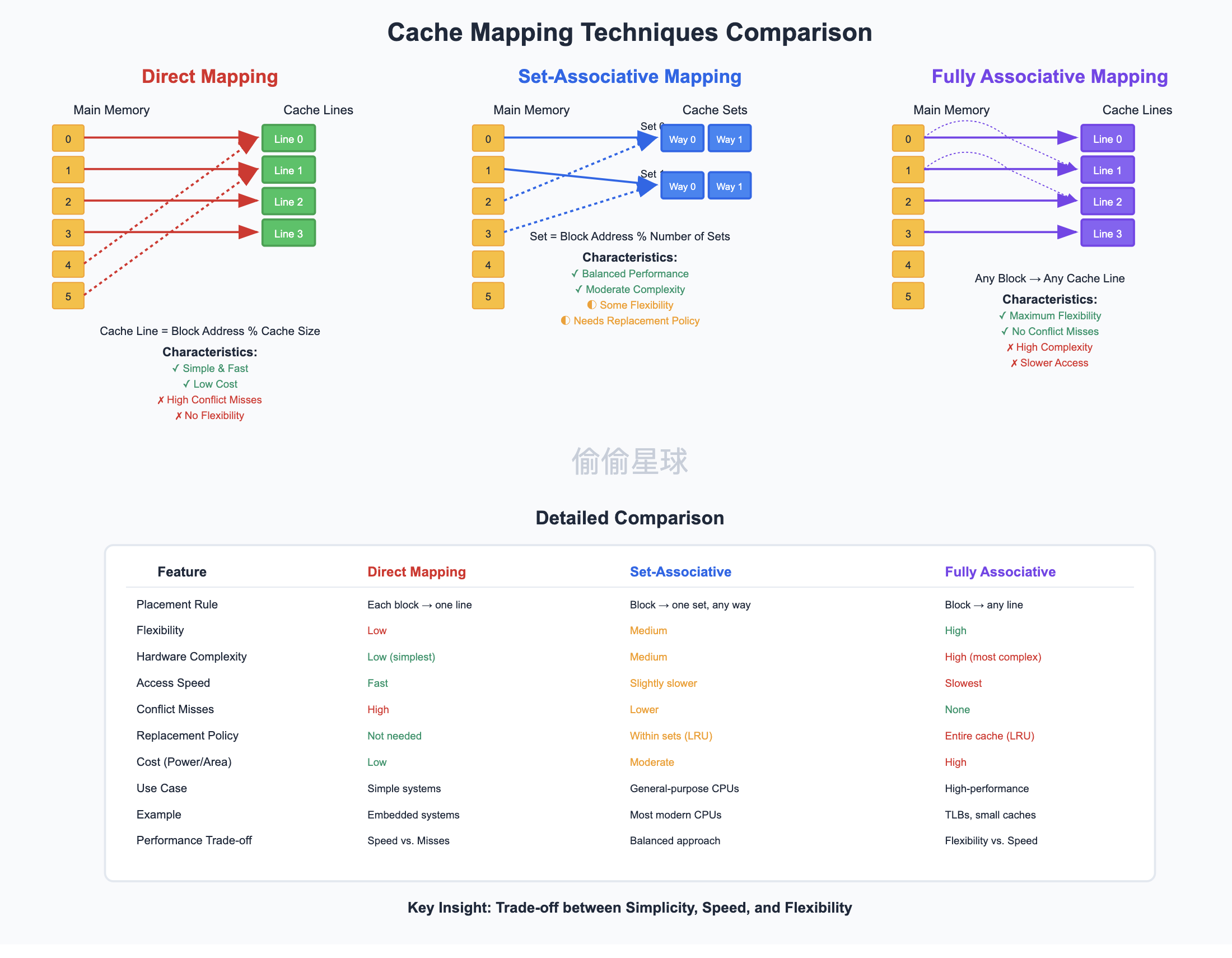
Direct Mapping（直接映射）

Direct Mapping is a simple cache mapping technique used in computer architecture to determine where a memory block will be placed in the cache.

🔧 Definition:
In Direct Mapping, each block of main memory maps to exactly one cache line. The mapping is usually done using:

Cache Line Index = (Main Memory Block Address) mod (Number of Cache Lines)

This makes it easy and fast to locate data in the cache, but can lead to many conflicts if multiple blocks map to the same cache line.

✅ Advantages:

Simple and fast implementation
Low hardware complexity

❌ Disadvantages:

High conflict rate: Two different memory blocks mapping to the same line will continuously evict each other
Low flexibility compared to other mapping techniques (e.g., set-associative)

🧠 Example:
If a cache has 8 lines (0 to 7), and a block from main memory has address 24:

Cache Line = 24 mod 8 = 0

So this block will always be placed in cache line 0.

Summary:
Direct Mapping provides fast and simple cache access, but is prone to frequent conflicts.

Set- Associative Mapping（组相连映射）

Set-Associative Mapping is a cache mapping technique that combines the benefits of both Direct Mapping and Fully Associative Mapping to balance performance and complexity.

🔧 Definition:
In Set-Associative Mapping, the cache is divided into multiple sets, and each set contains multiple cache lines (ways). A block from main memory maps to exactly one set, but can be placed in any line (way) within that set.

The set is selected using:

Set Index = (Main Memory Block Address) mod (Number of Sets)

Within the set, placement and replacement follow policies like Least Recently Used (LRU) or Random.

✅ Advantages:

Lower conflict rate than Direct Mapping
More flexible placement within sets
Good balance between speed and cache hit rate

❌ Disadvantages:

More complex hardware than Direct Mapping
Slightly slower lookup due to checking multiple lines in a set

🧠 Example:
If a cache has 4 sets, each with 2 lines (2-way set-associative), and a memory block with address 12:

Set Index = 12 mod 4 = 0

The block can be placed in either of the 2 lines in Set 0.

Summary:
Set-Associative Mapping provides a balanced approach with better conflict resolution than Direct Mapping and less complexity than Fully Associative Mapping.

Full Associative Mapping（全相联映射）

Full Associative Mapping is a cache mapping technique in which a memory block can be placed in any cache line, offering maximum flexibility and minimal conflict.

🔧 Definition:
In Full Associative Mapping, there are no restrictions on where a block can be placed in the cache. Any block from main memory can be stored in any cache line.

To find a block, the cache must search all lines using comparators that match tags.

✅ Advantages:

No conflict misses (except when cache is full)
Best flexibility in placement
Highest cache hit potential

❌ Disadvantages:

Complex hardware: Requires searching the entire cache in parallel
Slower access time due to tag comparisons
Expensive in terms of power and chip area

🧠 Example:
If a cache has 8 lines, and a block from memory has address 0x2F, it can be placed in any one of the 8 lines. When checking for a hit, the cache must compare the block’s tag with the tags of all 8 lines.

Summary:
Full Associative Mapping provides maximum flexibility and minimal conflict, but comes with higher hardware cost and slower lookup times.

Comparison of Cache Mapping Techniques

Feature	Direct Mapping	Set-Associative Mapping	Full Associative Mapping
Placement Rule	Each block maps to one line	Each block maps to one set, can go into any line in that set	Each block can go into any line in the cache
Flexibility	Low	Medium	High
Hardware Complexity	Low (simplest)	Medium	High (most complex)
Access Speed	Fast	Slightly slower	Slowest (due to parallel comparisons)
Conflict Misses	High	Lower than Direct Mapping	None (except capacity misses)
Replacement Policy	Not needed (only one line)	Needed within each set (e.g., LRU)	Needed for the entire cache (e.g., LRU)
Cost (Power/Area)	Low	Moderate	High
Use Case Suitability	Simple, low-power systems	General-purpose CPUs	High-performance or critical systems

Cache

Cache is a small, high-speed memory that stores frequently used data to speed up access. It sits between the CPU and main memory to reduce latency. It enables fast program access to frequently used addresses.

Non-blocking Cache（非阻塞缓存）

A Non-blocking Cache allows the CPU to continue processing other instructions while waiting for a cache miss to be resolved.
It supports multiple outstanding memory requests simultaneously.
This improves overall system performance by reducing CPU idle time.
Non-blocking caches are especially useful in out-of-order execution and superscalar processors.
They often use structures like Miss Status Handling Registers (MSHRs) to track pending requests.

非阻塞缓存允许 CPU 在等待缓存未命中（Cache Miss）处理完成的同时继续执行其他指令。
它支持多个未完成的内存请求同时存在。
这通过减少 CPU 空闲时间来提升系统整体性能。
非阻塞缓存在乱序执行和超标量处理器中尤为重要。
它通常使用如 未命中状态处理寄存器（Miss Status Handling Registers, MSHRs） 的结构来追踪未完成的请求。

Superscalar Architecture（超标量架构）

Superscalar Architecture is a CPU design that allows the processor to fetch, decode, and execute multiple instructions simultaneously during each clock cycle.
It achieves this by using multiple pipelines and parallel execution units (e.g., ALUs, FPUs).
This architecture increases instruction-level parallelism (ILP), boosting performance without raising the clock speed.
Superscalar CPUs include features like out-of-order execution, register renaming, and branch prediction to handle dependencies and control flow efficiently.
Examples of superscalar processors include modern Intel and AMD CPUs.

🔍 TLB (Translation Lookaside Buffer)

TLB stands for Translation Lookaside Buffer. It is a small, fast cache used in the memory management unit (MMU) of a computer’s CPU to improve the speed of virtual-to-physical address translation.

📌 Why is TLB needed?

When a CPU accesses memory using a virtual address, it must be translated into a physical address using the page table. This translation is time-consuming. The TLB stores recent translations, so if the virtual address has been accessed recently, the translation can be retrieved quickly without accessing the full page table.

✅ Key Characteristics

Cache for page table entries
Reduces page table access time
Typically contains 64 to 512 entries
Can be fully associative, set-associative, or direct-mapped

📈 How it works

CPU generates a virtual address
MMU checks the TLB for the virtual page number (VPN)
If found (TLB hit): use the cached physical page number (PPN)
If not found (TLB miss): access the page table, then update the TLB

🧠 TLB Hit vs TLB Miss

Event	Description
TLB Hit	The virtual address is found in the TLB → Fast address translation
TLB Miss	The virtual address is not found in the TLB → Page table lookup is required

🧮 Example

Let’s say the CPU wants to access virtual address 0x00403ABC:

VPN = top bits of address → check if TLB has entry
If yes → get PPN and combine with offset → access physical memory
If no → consult page table → update TLB → then access memory

🔄 TLB Replacement Policy

When the TLB is full, and a new entry must be loaded, a replacement policy is used, such as:

Least Recently Used (LRU)
Random replacement

🚀 Summary

TLB significantly improves performance of memory access.
Acts as a fast cache for recent address translations.
Helps bridge the speed gap between the CPU and memory systems.

Page Table

In computer architecture, a Page Table is a data structure used by the virtual memory system to manage the mapping between virtual addresses and physical addresses.

🧠 What is Virtual Memory?

Virtual memory allows a program to use a large, continuous address space even if the physical memory (RAM) is smaller. The CPU generates virtual addresses, which must be translated into physical addresses before accessing actual memory.

📘 What is a Page Table?

A Page Table stores the mapping between virtual pages and physical frames. Each entry in the page table is called a Page Table Entry (PTE) and contains information such as:

Frame Number: the physical frame corresponding to the virtual page.
Valid/Invalid Bit: indicates if the mapping is valid.
Protection Bits: control read/write permissions.
Dirty Bit: indicates if the page has been modified.
Accessed Bit: indicates if the page has been accessed recently.

🧾 Example Structure

Virtual Page Number	Physical Frame Number	Valid Bit	Protection
0	5	1	Read/Write
1	2	1	Read-only
2	-	0	-

🧮 Address Translation Steps

The CPU generates a virtual address.
The virtual address is divided into:
- Page Number
- Offset
The Page Number is used to index into the Page Table.
The Page Table Entry provides the Frame Number.
The Physical Address is formed by combining the Frame Number and the Offset.

🛑 Page Fault

If the Valid Bit is 0, the page is not currently in memory. This triggers a Page Fault, and the operating system must load the page from disk into RAM.

🧭 Types of Page Tables

Single-Level Page Table: Simple but not scalable for large address spaces.
Multi-Level Page Table: Reduces memory usage by using a tree-like structure.
Inverted Page Table: Indexes by physical frame instead of virtual page.
Hashed Page Table: Used in systems with large address spaces (like 64-bit).

📌 Summary

Page Tables are essential for translating virtual to physical addresses.
They enable memory protection, process isolation, and efficient memory use.
Optimized with techniques like TLB (Translation Lookaside Buffer) to speed up address translation.

🧩 3 Types of Cache Misses

In computer architecture, a cache miss occurs when the data requested by the CPU is not found in the cache, requiring access to a slower memory level (like RAM). There are three main types of cache misses:

🧠 Summary Table

Type	Cause	Possible Solution
Compulsory Miss	First-time access to a block	Prefetching, larger block size
Capacity Miss	Cache too small for working set	Larger cache, better algorithms
Conflict Miss	Blocks map to the same cache location	Higher associativity, alignment

1. Compulsory Miss (a.k.a. Cold Miss)

🔹 What is it?

Occurs the first time a block is accessed and has never been loaded into the cache before.

🧠 Cause:

Cache is empty or data is accessed for the first time.

📌 Example:

Accessing array A[0] for the first time → not in cache → compulsory miss

✅ Solution:

Prefetching
Larger block size (to bring in more adjacent data)

2. Capacity Miss

🔹 What is it?

Happens when the cache cannot contain all the needed data, and a previously loaded block gets evicted due to limited size.

🧠 Cause:

The working set is larger than the cache.

📌 Example:

Looping through a large dataset that exceeds cache size → older blocks are evicted → miss

✅ Solution:

Increase cache size
Optimize algorithm locality

3. Conflict Miss (a.k.a. Collision Miss)

🔹 What is it?

Occurs when multiple blocks map to the same cache line (in set-associative or direct-mapped caches), causing unnecessary evictions.

🧠 Cause:

Limited associativity in the cache
Poor address mapping

📌 Example:

Accessing addresses A and B that both map to cache set 3 → one evicts the other → conflict miss

✅ Solution:

Increase associativity
Use fully associative cache
Better hash functions or memory alignment

🔗 Four Types of Data Dependencies in Computer Architecture

In pipelined processors, data dependencies occur when instructions depend on the results of previous instructions. These dependencies can cause pipeline hazards and impact instruction-level parallelism.

There are four types of data dependencies:

📊 Summary Table

Type	Abbreviation	Cause	Solution
Flow Dependency	RAW	Read after write	Forwarding, Stall
Anti Dependency	WAR	Write after read	Register renaming
Output Dependency	WAW	Write after write	Register renaming, in-order commit
Control Dependency	–	Depends on branch outcome	Branch prediction, speculation

1. Flow Dependency (Read After Write, RAW)

🔹 What is it?

Occurs when an instruction needs to read a value that has not yet been written by a previous instruction.

🧠 Cause:

The second instruction depends on the result of the first.

📌 Example:

I1: R1 ← R2 + R3
I2: R4 ← R1 + R5   ; RAW: I2 reads R1 before I1 writes it

✅ Solution:

Forwarding/Bypassing
Stalling the pipeline

2. Anti Dependency (Write After Read, WAR)

🔹 What is it?

Occurs when a later instruction writes to a location that a previous instruction still needs to read from.

🧠 Cause:

The second instruction must not overwrite the value too early.

📌 Example:

I1: R4 ← R1 + R2   ; Reads R1
I2: R1 ← R3 + R5   ; WAR: I2 writes R1 before I1 finishes reading

✅ Solution:

Register renaming

3. Output Dependency (Write After Write, WAW)

🔹 What is it?

Occurs when two instructions write to the same destination, and the final result must reflect the correct write order.

🧠 Cause:

Later instruction must not overwrite an earlier write out of order.

📌 Example:

I1: R1 ← R2 + R3
I2: R1 ← R4 + R5   ; WAW: I2 writes R1 before I1 completes

✅ Solution:

Register renaming
In-order commit in out-of-order execution

4. Control Dependency

🔹 What is it?

Occurs when the execution of an instruction depends on the outcome of a branch.

🧠 Cause:

It’s not clear whether to execute the instruction until the branch is resolved.

📌 Example:

I1: if (R1 == 0) goto LABEL
I2: R2 ← R3 + R4   ; Control dependent on I1

✅ Solution:

Branch prediction
Speculative execution

Microprogramming（微程序设计）

Microprogramming is a method of implementing a CPU’s control unit using a sequence of microinstructions stored in a special memory called control memory.
Each microinstruction specifies low-level operations like setting control signals, reading/writing registers, or ALU actions.
It acts as an intermediate layer between machine instructions and hardware control signals.
There are two types of control units: hardwired control and microprogrammed control — the latter is easier to modify and extend.
Microprogramming was widely used in classic CISC architectures like IBM System/360.

Snoopy Cache（监听式缓存）

Snoopy Cache is a cache coherence protocol used in multiprocessor systems to maintain data consistency among multiple caches.
Each cache monitors (or “snoops”) a shared communication bus to detect if other processors are reading or writing a memory block it has cached.
If a write is detected, the snooping cache can invalidate or update its own copy to keep data coherent.
This ensures that all processors work with the most recent version of data.
Common snoopy-based protocols include MSI, MESI, and MOESI.

Snoopy Cache（监听式缓存）是一种用于多处理器系统的缓存一致性协议，用于保持多个缓存之间的数据一致性。
每个缓存会监听（snoop）共享总线，检测其他处理器是否在读取或写入它缓存中的数据块。
当检测到写操作时，监听缓存会更新或无效化自己的副本，以保持数据的一致性。
这样可以确保所有处理器使用的都是最新版本的数据。
常见的监听式协议包括 MSI、MESI 和 MOESI 协议。

Out-of-order Execution (乱序执行)

Out-of-order execution is a technique used in modern processors to improve performance by allowing instructions to be executed out of the order they appear in the program.
Instead of waiting for earlier instructions to complete (which might be delayed due to data hazards or memory stalls), the CPU executes instructions that are ready and independent of others.
This reduces idle CPU time and increases throughput by utilizing all available execution units.
Dependencies between instructions are tracked, and results are committed in the correct order.
Out-of-order execution is common in superscalar processors and is part of dynamic instruction scheduling.

乱序执行是一种现代处理器中常用的技术，通过允许指令按非顺序的方式执行来提升性能。
CPU 不必等待前面的指令完成（这些指令可能因为数据依赖或内存延迟而被拖慢），而是执行那些准备好且相互独立的指令。
这样可以减少CPU空闲时间并增加吞吐量，充分利用所有可用的执行单元。
指令之间的依赖关系会被追踪，结果会按正确的顺序提交。
乱序执行在超标量处理器中很常见，并且是动态指令调度的一部分。

DMA (Direct Memory Access)

DMA stands for Direct Memory Access, a feature that allows certain hardware components (like disk controllers or network cards) to transfer data directly to/from main memory without involving the CPU.
This improves system efficiency by freeing the CPU from managing large or repetitive data transfers.
A DMA controller handles the data movement and signals the CPU when the transfer is complete.
DMA is commonly used for tasks like disk I/O, audio/video streaming, and network communication.
It helps achieve high-speed data transfer with minimal CPU overhead.

DMA 是 直接内存访问（Direct Memory Access） 的缩写，是一种允许某些硬件组件（如磁盘控制器或网卡）在不经过 CPU 的情况下直接与主存进行数据传输的技术。
它通过减轻 CPU 的数据搬运负担，提高了系统效率。
数据传输由一个 DMA 控制器负责，传输完成后会通知 CPU。
DMA 广泛应用于 磁盘 I/O、音视频流处理 和 网络通信 等领域。
它能以极低的 CPU 开销实现高速数据传输。

RISC (Reduced Instruction Set Computing)

RISC stands for Reduced Instruction Set Computing, a CPU design strategy that uses a small set of simple and fast instructions.
Each instruction typically executes in one clock cycle, allowing efficient pipelining and parallelism.
RISC emphasizes hardware simplicity, fixed instruction length, and a load/store architecture.
It is well-suited for modern compilers and high-performance applications.
Examples: ARM, RISC-V, MIPS.

RISC 是 精简指令集计算（Reduced Instruction Set Computing） 的缩写，是一种使用少量简单指令的 CPU 设计理念。
每条指令通常在一个时钟周期内完成，便于实现流水线和并行处理。
RISC 强调硬件简化、固定长度指令以及Load/Store 架构。
这种架构非常适合现代编译器和高性能应用。
代表架构：ARM、RISC-V、MIPS。

CISC (Complex Instruction Set Computing)

CISC stands for Complex Instruction Set Computing, which uses a large and versatile set of instructions, where some instructions perform multi-step operations.
This design reduces the number of instructions per program but increases the complexity of the CPU.
CISC instructions often have variable lengths and require multiple clock cycles to execute.
It was originally designed to minimize memory usage and support simpler compilers.
Example: x86 architecture (Intel, AMD).

CISC 是 复杂指令集计算（Complex Instruction Set Computing） 的缩写，采用数量多、功能强的指令集，其中一些指令能完成多个低层次操作。
这种设计可以减少程序中所需的指令数量，但会增加 CPU 的实现复杂度。
CISC 指令通常是不固定长度，并且执行时可能需要多个时钟周期。
它最初为了减少内存使用、便于早期编译器设计而提出。
代表架构：x86 架构（如 Intel 和 AMD 处理器）。

SIMD (Single Instruction, Multiple Data)

SIMD stands for Single Instruction, Multiple Data, a parallel computing model where one instruction operates on multiple data elements simultaneously.
It is especially useful for tasks like image processing, audio/video encoding, machine learning, and scientific computing.
SIMD improves performance by exploiting data-level parallelism.
Modern CPUs include SIMD instruction sets such as SSE, AVX (Intel/AMD), and NEON (ARM).
It is a core concept in vector processing and used in GPUs as well.

SIMD 是 单指令多数据流（Single Instruction, Multiple Data） 的缩写，是一种并行计算模型，其中一条指令可以同时作用于多个数据元素。
它非常适用于图像处理、音视频编解码、机器学习和科学计算等场景。
SIMD 通过挖掘数据级并行性（Data-level Parallelism）来提升性能。
现代 CPU 提供了 SIMD 指令集，如 SSE、AVX（Intel/AMD）和 NEON（ARM）。
它是向量处理（Vector Processing）的核心思想，并广泛用于 GPU 中。

4. Formal Language & Automata

Regular Grammar

A Regular Grammar is the simplest type of grammar in the Chomsky hierarchy. It is used to define regular languages, which can also be recognized by finite automata. Regular grammars are widely used in lexical analysis, pattern matching, and simple parsing tasks.

📘 Definition

A Regular Grammar is a type of context-free grammar (CFG) with special restrictions on its production rules. It consists of:

A finite set of non-terminal symbols
A finite set of terminal symbols
A start symbol
A finite set of production rules

🧾 Types of Regular Grammar

There are two forms of regular grammars:

Right-Linear Grammar

All production rules are of the form:

$A \rightarrow aB$
$A \rightarrow a$
$A \rightarrow \varepsilon$ (optional for generating empty string)

Where:

$A, B$ are non-terminal symbols
$a$ is a terminal symbol

✅ This is the most common form used to generate regular languages.

Left-Linear Grammar

All production rules are of the form:

$A \rightarrow Ba$
$A \rightarrow a$
$A \rightarrow \varepsilon$

Both right-linear and left-linear grammars generate regular languages, but mixing them is not allowed in regular grammar.

🧮 Example of a Right-Linear Grammar

Let’s define a grammar for the regular language $L = { a^n b \mid n \geq 0 }$:

Non-terminals: ${S, A}$
Terminals: ${a, b}$
Start symbol: $S$
Production rules:

S → aS  
S → b

This generates strings like:

b
ab
aab
aaab, etc.

🤖 Equivalent Automata

Every regular grammar corresponds to a finite automaton, and vice versa:

Model	Description
Regular Grammar	Generates strings by rules
Finite Automaton	Accepts strings by state transitions

So, regular grammar and finite automaton are equivalent in expressive power.

📊 Closure Properties

Regular grammars inherit all the closure properties of regular languages:

✅ Union
✅ Concatenation
✅ Kleene Star
✅ Intersection with regular sets
✅ Complement

🚫 Limitations

Cannot handle nested structures (e.g., balanced parentheses)
Cannot count or match multiple dependencies (e.g., $a^n b^n$)

✅ Summary

Feature	Regular Grammar
Structure	Right- or left-linear rules
Generates	Regular languages
Equivalent to	Finite Automaton
Used in	Lexical analysis, pattern matching
Can generate $a^n$	✅ Yes
Can generate $a^n b^n$	❌ No

Regular Language

A Regular Language is a class of formal languages that can be recognized by finite automata. It can be described by:

Deterministic Finite Automata (DFA)
Non-deterministic Finite Automata (NFA)
Regular expressions

If a language can be represented using any of the above methods, it is a regular language.

🔹 Examples

Language of all strings over {a, b} that contain only a:
```
L = { ε, a, aa, aaa, ... } = a*
```
Language of all strings that start with a and end with b:
```
L = a(a|b)*b
```
Language of all strings with even number of 0s over {0,1}:
- This can be recognized by a DFA with two states toggling on 0.

They can be expressed using regular expressions, and there is an equivalence between:
```
DFA ⇄ NFA ⇄ Regular Expression
```

Non-Regular Languages

Some languages cannot be described by regular expressions or finite automata. For example:

L = { aⁿbⁿ | n ≥ 0 }

This language requires memory to keep track of the number of as and bs, which finite automata do not have.

To prove that a language is not regular, we can use the Pumping Lemma, which states:

If a language L is regular, there exists an integer p > 0 (pumping length) such that any string s ∈ L with length ≥ p can be split into s = xyz such that:

|y| > 0
|xy| ≤ p
For all i ≥ 0, the string xyⁱz ∈ L

If no such decomposition exists for a string, the language is not regular.

Closure Properties of Regular Languages

🔹 What is “Closure”?

In automata theory, a class of languages is said to be closed under an operation if applying that operation to languages in the class results in a language that is also in the class.

For regular languages, they are closed under many operations. This means if you take regular languages and apply these operations, the result will still be a regular language.

🔹 Closure Under Common Operations

Operation	Description	Result
Union	If L₁ and L₂ are regular, then L₁ ∪ L₂ is also regular.	✅ Regular
Intersection	If L₁ and L₂ are regular, then L₁ ∩ L₂ is also regular.	✅ Regular
Complement	If L is regular, then its complement ¬L is also regular.	✅ Regular
Concatenation	If L₁ and L₂ are regular, then L₁L₂ is also regular.	✅ Regular
Kleene Star	If L is regular, then L* (zero or more repetitions) is also regular.	✅ Regular
Reversal	If L is regular, then the reverse of L is also regular.	✅ Regular
Difference	If L₁ and L₂ are regular, then L₁ - L₂ is also regular.	✅ Regular
Homomorphism	Applying a homomorphism to a regular language gives a regular language.	✅ Regular
Inverse Homomorphism	Inverse images of regular languages under homomorphisms are regular.	✅ Regular
Substitution	Regular languages are closed under substitution with regular languages.	✅ Regular

🔹 Example: Union Closure

Let:

L₁ = { w | w contains only a’s } = a*
L₂ = { w | w contains only b’s } = b*

Then:

L₁ ∪ L₂ = { w | w contains only a’s or only b’s } = a* ∪ b*
This is still a regular language.

🔹 Why Closure is Useful

Closure properties help us construct complex regular languages from simpler ones.
They are essential in proving properties of languages.
They are used in compiler design, regex engines, and automated verification.

🤖 DFA (Deterministic Finite Automaton)

🔹 Definition

A DFA is a type of finite automaton used to recognize regular languages. It reads an input string symbol by symbol, and at any point in time, it is in exactly one state.

A DFA is defined as a 5-tuple:

DFA = (Q, Σ, δ, q₀, F)

Where:

Q → Finite set of states
Σ → Finite set of input symbols (alphabet)
δ → Transition function: δ : Q × Σ → Q
q₀ → Start state, where the computation begins (q₀ ∈ Q)
F → Set of accepting/final states (F ⊆ Q)

🔹 Characteristics

Deterministic: For every state q ∈ Q and every input symbol a ∈ Σ, there is exactly one transition defined:
δ(q, a) = q’
No epsilon (ε) transitions: Input must be read one symbol at a time
DFA always knows what to do next

🔹 Example DFA

Let’s define a DFA that accepts all strings over {0,1} that end with 01.

Q = {q0, q1, q2}
Σ = {0, 1}
q₀ = q0
F = {q2}

Transition table:

Current State	Input	Next State
q0	0	q1
q0	1	q0
q1	0	q1
q1	1	q2
q2	0	q1
q2	1	q0

This DFA accepts strings like: 01, 1001, 1101, etc.

🔹 DFA vs NFA

Feature	DFA	NFA
Transition	One unique next state	May have multiple next states
ε-transitions	Not allowed	Allowed
Simplicity	Easier to implement	Easier to design
Power	Same (both recognize regular languages)

🔹 Applications

Lexical analysis (token recognition)
Pattern matching (e.g., grep, regex)
Protocol design
Digital circuits

🔄 NFA (Nondeterministic Finite Automaton)

🔹 Definition

An NFA is a type of finite automaton used to recognize regular languages, just like a DFA. The key difference is that multiple transitions are allowed for the same input from a single state, and ε-transitions (transitions without consuming input) are permitted.

An NFA is formally defined as a 5-tuple:

NFA = (Q, Σ, δ, q₀, F)

Where:

Q → Finite set of states
Σ → Finite set of input symbols (alphabet)
δ → Transition function: δ : Q × (Σ ∪ {ε}) → 2^Q
q₀ → Start state, q₀ ∈ Q
F → Set of accepting/final states, F ⊆ Q

🔹 Characteristics

Non-deterministic:
- From a given state and input, the NFA can go to multiple next states.
- The NFA accepts an input string if at least one possible path leads to an accepting state.
ε-transitions allowed: The machine can move without reading input.
Can be in multiple states at once during computation.

🔹 Example NFA

Let’s define an NFA that accepts strings over {0,1} ending in 01.

Q = {q0, q1, q2}
Σ = {0, 1}
q₀ = q0
F = {q2}

Transition table:

Current State	Input	Next States
q0	0	{q0, q1}
q0	1	{q0}
q1	1	{q2}
q2	0,1	∅

In this NFA, from q0, if we read 0, we can either stay in q0 or go to q1.

🔹 NFA vs DFA

Feature	NFA	DFA
Transitions	Can go to multiple states	Only one next state
ε-transitions	Allowed	Not allowed
Execution	Can explore multiple paths in parallel	Only one deterministic path
Implementation	More complex	Easier
Expressive Power	Same – both recognize regular languages

💡 Every NFA can be converted into an equivalent DFA (subset construction), though the DFA may have exponentially more states.

🔹 Applications

Easier to design than DFA for complex patterns
Used in regular expression engines
Foundations for parser generators and compiler design

Finite-State Machine (FSM)

A Finite-State Machine (FSM) is a computational model used to design and describe the behavior of digital systems, software, or processes that are dependent on a sequence of inputs and a finite number of internal states.

🧠 Key Concepts

Term	Description
State	A unique configuration or condition of the system at a given time.
Input	External data or signal that triggers a transition.
Transition	The process of moving from one state to another.
Initial State	The state in which the FSM starts.
Final State(s)	Some FSMs may have one or more accepting states that signify a successful process.

🛠 Types of FSM

Deterministic Finite Automaton (DFA)
- Each state has exactly one transition for each possible input.
- There is no ambiguity in state transitions.
Nondeterministic Finite Automaton (NFA)
- A state can have multiple transitions for the same input.
- May include ε-transitions (transitions without input).

⚙️ Components of an FSM

An FSM is formally defined as a 5-tuple:

$$
M = (Q, \Sigma, \delta, q_0, F)
$$

🧭 How It Works (Example)

Suppose we have an FSM that accepts binary strings ending in 01.

States: S0 (start), S1 (seen 0), S2 (accepting, seen 01)
Input: 0, 1
Transitions:
- From S0, on 0 → S1
- From S1, on 1 → S2
- From S2, on 0 → S1, on 1 → S0 (reset if wrong pattern)

📦 Applications

Lexical analyzers (compilers)
Protocol design
Game development (e.g., AI behavior)
Digital circuit design
Control systems

Pumping Lemma for regular languages

The Pumping Lemma for regular languages is an important tool in formal language and automata theory, used to prove that a given language is not regular. The pumping lemma provides a “pumping” property, which means that certain strings in a regular language can be repeated (or “pumped”) under specific conditions without changing whether the string belongs to the language.

The pumping lemma mainly applies to regular languages. It states:
If a language is regular, then there exists a constant $p$ (called the pumping length), such that for any string $s \in L$ (where $s$ belongs to language $L$) with length greater than or equal to $p$, it is possible to divide $s$ into the following three parts:

$s = xyz$, where:
- $x$ is a prefix of $s$ (possibly empty).
- $y$ is the part that can be “pumped”, and $|y| > 0$.
- $z$ is a suffix of $s$ (possibly empty).

Moreover, for any $i \geq 0$, the string $xy^i z$ must also belong to the language $L$. That is, the substring $y$ can be repeated any number of times without affecting whether $s$ belongs to $L$.

Pumping Lemma for CFLs

The Pumping Lemma for Context-Free Languages (CFLs) states that for any context-free language $L$, if $L$ is infinite, then there exists a constant $p$ (pumping length), such that for every string $s \in L$ with length greater than or equal to $p$, the string $s$ can be divided into five parts $s = uvwxy$, satisfying the following conditions:

For all $i \geq 0$, $uv^i w x^i y \in L$.
$|v| + |x| > 0$ (i.e., $v$ and $x$ are not both empty).
$|vwx| \leq p$ (the total length of $v$, $w$, and $x$ does not exceed the pumping length $p$).

We assume that $L$ is an infinite context-free language. Since $L$ is a context-free language, based on the structural properties of context-free grammars, it corresponds to a pushdown automaton (PDA). This PDA must satisfy one condition: it can “pump” strings, i.e., repeat certain parts of the string while keeping the resulting string within the language $L$.

According to the pumping lemma assumption, there exists a pumping length $p$, such that for all strings $s \in L$ with length greater than or equal to $p$, the string $s$ can be decomposed as $s = uvwxy$, satisfying the following conditions:

$|vwx| \leq p$
$|v| + |x| > 0$

Context-free languages can be generated by context-free grammars (CFGs) or recognized by pushdown automata (PDAs). We use these structures to demonstrate the pumping lemma.

For any string $s \in L$ with length greater than or equal to $p$, it must be generated by derivation using a context-free grammar.
Since $L$ is infinite, there exists a derivation tree for some parts that can be broken down into five parts $uvwxy$, where:
- $v$ and $x$ are the parts that can be “pumped” or repeated.
- The total length of $v$ and $x$ does not exceed $p$.
- This means that for some appropriate $i$, $v$ and $x$ can be repeated without breaking the structure of the language.

The proof here also involves the Pigeonhole Principle, which is not elaborated on in detail.

Based on the structure of context-free languages, the string $s$ can be decomposed as $s = uvwxy$, satisfying the following conditions:

$|vwx| \leq p$, which means the total length of $v$ and $x$ does not exceed the pumping length $p$; their lengths are finite.
$|v| + |x| > 0$, which means $v$ and $x$ cannot both be empty.

According to the pumping lemma, we know that if we “pump” the parts $v$ and $x$ of the string $s$, i.e., repeat them multiple times, then the new string $uv^i w x^i y$ will still belong to the language $L$, for all $i \geq 0$.

According to the pumping lemma assumption, for all $i \geq 0$, $uv^i w x^i y \in L$. This means that by increasing the number of repetitions of parts $v$ and $x$, the string remains within the language $L$.

The key to this process is that through appropriate decomposition and pumping operations, the structure of the language remains unchanged, and therefore it can be accepted by a context-free grammar or pushdown automaton.

Using the pumping lemma, we can prove that some languages are not context-free. A proof by contradiction is often used to show that a language does not satisfy the requirements of a context-free language. By choosing an appropriate string and assuming it satisfies the conditions of the pumping lemma, we can show that certain operations cause the resulting string to no longer belong to the language, thus concluding that the language is not context-free.

Using the pumping lemma, we can prove that certain languages are not context-free by contradiction. Suppose we want to prove that a language $L$ is not context-free. The process usually involves the following steps:

Assume that $L$ is a context-free language and that it satisfies the pumping lemma.
Choose a string $s \in L$ with length greater than or equal to the pumping length $p$, then decompose it as $s = uvwxy$ and apply the pumping lemma.
Expand $uv^i w x^i y$ and prove that for some values of $i$, $uv^i w x^i y \notin L$, thus leading to a contradiction.
Conclude that $L$ is not a context-free language.

Example: Prove that $L = { a^n b^n c^n \mid n \geq 0 }$ is not a context-free language.

We use the pumping lemma for context-free languages to prove that $L = { a^n b^n c^n \mid n \geq 0 }$ is not context-free.

Assume $L$ is a context-free language:
Assume that $L$ is a context-free language and that a pumping length $p$ exists. According to the pumping lemma, any string $s$ with length greater than or equal to $p$ can be decomposed as $s = uvwxy$, where $|vwx| \leq p$ and $|v| + |x| > 0$.
Choose the string $s = a^p b^p c^p$:
Choose the string $s = a^p b^p c^p$, which clearly belongs to $L$, and its length $|s| = 3p \geq p$.
Decompose the string $s$:
According to the pumping lemma, $s = uvwxy$, where $|vwx| \leq p$ and $|v| + |x| > 0$. Since $|vwx| \leq p$, it can only span one portion of the string (i.e., the $a^n$, $b^n$, or $c^n$ part). Also, since $|v| + |x| > 0$, $v$ and $x$ must include some repeating characters.
Apply the pumping lemma:
According to the pumping lemma, for all $i \geq 0$, $uv^i w x^i y$ should still belong to $L$. However, if we choose $i > 1$, we get a mismatched string such as $uv^2 w x^2 y$. This string would no longer maintain the same number of as, bs, and cs, and thus would not belong to $L$.
Reach a contradiction:
Therefore, we conclude that $L$ cannot be a context-free language because the result from the pumping lemma contradicts the definition of $L$.

The pumping lemma for context-free languages demonstrates certain properties of languages by decomposing and repeating parts of their strings. It provides a method to prove by contradiction that certain languages are not context-free.

Context-Free Language (CFL)

A Context-Free Language (CFL) is a type of formal language that can be generated by a Context-Free Grammar (CFG). It is an essential concept in the theory of computation and plays a major role in compiler design and parsing.

📘 What is a Context-Free Grammar (CFG)?

A Context-Free Grammar is a set of recursive rewriting rules (productions) used to generate strings in a language. A CFG is formally defined as a 4-tuple:

$$
G = (V, \Sigma, R, S)
$$

Where:

$V$: A finite set of variables (non-terminal symbols)
$\Sigma$: A finite set of terminal symbols (alphabet of the language)
$R$: A finite set of production rules, each of the form $A \rightarrow \gamma$, where $A \in V$ and $\gamma \in (V \cup \Sigma)^*$
$S$: The start symbol, $S \in V$

🧠 Key Characteristics of CFLs

The left-hand side of every production rule in a CFG has exactly one non-terminal.
A string belongs to the CFL if it can be derived from the start symbol using the rules.
CFLs are more powerful than regular languages, but less powerful than context-sensitive languages.

🧮 Example of a Context-Free Grammar

Let’s define a CFG for the language $L = { a^n b^n \mid n \geq 0 }$:

Grammar:

$V = { S }$
$\Sigma = { a, b }$
Production Rules:
- $S \rightarrow aSb$
- $S \rightarrow \varepsilon$ (epsilon, the empty string)
$S$: start symbol

This grammar generates:

$\varepsilon$
$ab$
$aabb$
$aaabbb$, etc.

📊 Closure Properties of CFLs

Operation	Closed under?
Union	✅ Yes
Concatenation	✅ Yes
Kleene Star	✅ Yes
Intersection	❌ No
Complement	❌ No

🖥 Recognizing CFLs with Pushdown Automata (PDA)

A Pushdown Automaton (PDA) is a computational model that recognizes context-free languages.
It is similar to a finite automaton but with an added stack, which allows it to store an unbounded amount of information.

CFLs are exactly the class of languages accepted by nondeterministic PDAs.

🚫 Not All Languages Are CFLs

Some languages are not context-free, for example:

$$
L = { a^n b^n c^n \mid n \geq 0 }
$$

No CFG can generate this language because it requires three-way balancing, which CFGs cannot handle.

🧪 Applications of CFLs

Programming languages (syntax parsing)
Compilers (syntax analysis)
Natural language processing
XML and structured data parsing

Pushdown Automaton (PDA)

A Pushdown Automaton (PDA) is a type of computational model that extends the finite automaton by adding a stack as memory. This additional memory allows it to recognize context-free languages (CFLs), which are more powerful than regular languages.

🧠 Intuition

A PDA reads input symbols one at a time, transitions between states based on the current input and the top of the stack, and can push or pop symbols from the stack.

Think of the stack as an unlimited memory that operates in LIFO (Last-In, First-Out) order.
The PDA uses the stack to keep track of nested or recursive patterns (e.g. matching parentheses).

🧱 Formal Definition

A PDA is a 7-tuple:

$$
M = (Q, \Sigma, \Gamma, \delta, q_0, Z_0, F)
$$

Where:

Symbol	Description
$Q$	A finite set of states
$\Sigma$	The input alphabet
$\Gamma$	The stack alphabet
$\delta$	The transition function: $Q \times (\Sigma \cup \varepsilon) \times \Gamma \rightarrow \mathcal{P}(Q \times \Gamma^*)$
$q_0$	The start state, $q_0 \in Q$
$Z_0$	The initial stack symbol, $Z_0 \in \Gamma$
$F$	A set of accepting (final) states, $F \subseteq Q$

🔁 Transition Function Explanation

The transition function:

$$
\delta(q, a, X) = { (q’, \gamma) }
$$

Means:

In state $q$, if the input symbol is $a$ (or $\varepsilon$), and the top of the stack is $X$,
Then the machine can:
- Move to state $q’$
- Replace $X$ with $\gamma$ on the stack (where $\gamma$ can be multiple symbols or empty)

🧮 Example: PDA for $L = { a^n b^n \mid n \geq 0 }$

We want to accept strings where the number of as equals the number of bs.

Idea:

Push A onto the stack for each a.
Pop A from the stack for each b.
Accept if the stack is empty at the end.

Step	Stack Operation
Read `a`	Push `A`
Read `b`	Pop `A`
Input done	Accept if stack empty

✅ Acceptance Criteria

There are two common acceptance methods for PDAs:

By final state: The PDA ends in an accepting state after reading the entire input.
By empty stack: The PDA’s stack is empty after reading the entire input.

Both methods define the same class of languages: context-free languages.

⚠️ Deterministic vs Nondeterministic PDA

Type	Description
NPDA	Nondeterministic PDA — accepts all CFLs
DPDA	Deterministic PDA — accepts only some CFLs

Not all context-free languages can be recognized by a deterministic PDA.

🔬 Applications

Parsing expressions in compilers
Syntax checking in programming languages (e.g., bracket matching)
Modeling recursive structures
Natural language processing (nested phrase structures)

Ambiguity of Grammar

In formal language theory, a grammar is said to be ambiguous if there exists at least one string that can be generated by the grammar in more than one way — specifically, it has more than one parse tree (or derivation).

📚 Definition

A context-free grammar (CFG) $G$ is ambiguous if there exists a string $w \in L(G)$ such that:

$w$ has two or more different parse trees, or
$w$ has two or more leftmost (or rightmost) derivations

🧠 Why Does Ambiguity Matter?

Ambiguous grammars are problematic in programming language design, especially during parsing, because a compiler may not know which interpretation is correct.
Some context-free languages are inherently ambiguous — no unambiguous CFG can generate them.

🧮 Example: An Ambiguous Grammar

Let’s define a simple grammar for arithmetic expressions:

E → E + E  
E → E * E  
E → (E)  
E → id

This grammar generates expressions like id + id * id, but it is ambiguous because:

It can be parsed as (id + id) * id
Or as id + (id * id)

Both are valid interpretations but yield different parse trees.

🌲 Two Different Parse Trees for id + id * id

1. Left-associative (Addition first)

    E
   /|\
  E + E
 |    |
id   E * E
     |   |
    id  id

2. Right-associative (Multiplication first)

       E
      /|\
     E * E
    |    |
   E + E id
  |   |
id  id

This shows ambiguity in structure and meaning.

🛠 Disambiguating a Grammar

To remove ambiguity, you can:

Introduce precedence and associativity rules (e.g., make * bind tighter than +)
Refactor the grammar to eliminate conflicting derivations

For example:

E  → E + T | T  
T  → T * F | F  
F  → (E) | id

Now:

* has higher precedence than +
Left associativity is enforced
This grammar is unambiguous

🔥 Inherently Ambiguous Languages

Some CFLs are inherently ambiguous, meaning no matter how you write the grammar, some strings will always have multiple parse trees.

Example language:

$$
L = { a^i b^j c^k \mid i = j \text{ or } j = k }
$$

This language is not inherently unambiguous because you can’t write a CFG for it that avoids ambiguity in all cases.

✅ Summary

Concept	Description
Ambiguity	A string has multiple parse trees or derivations in a grammar
Unambiguous CFG	A CFG where every string has only one parse tree
Inherently Ambiguous Language	A CFL for which no unambiguous grammar exists
Solution	Rewrite grammar with precedence/associativity or restructure rules

Turing Machine

A Turing Machine is a powerful abstract computational model introduced by Alan Turing in 1936. It forms the foundation of modern computer science and helps define the limits of what can be computed.

🧱 Definition

A Turing Machine (TM) is a 7-tuple:

$$
M = (Q, \Sigma, \Gamma, \delta, q_0, q_{\text{accept}}, q_{\text{reject}})
$$

Where:

Symbol	Meaning
$Q$	A finite set of states
$\Sigma$	The input alphabet (does not include the blank symbol `□`)
$\Gamma$	The tape alphabet (includes `□`, the blank symbol)
$\delta$	The transition function: $Q \times \Gamma \rightarrow Q \times \Gamma \times {L, R}$
$q_0$	The start state
$q_{\text{accept}}$	The accepting state
$q_{\text{reject}}$	The rejecting state (≠ $q_{\text{accept}}$)

🧠 How It Works

The machine has an infinite tape divided into cells, each holding one symbol from $\Gamma$.
A tape head reads and writes symbols on the tape and moves left (L) or right (R).
The machine starts in the start state $q_0$, with the tape containing the input string and blanks elsewhere.
Based on the current state and the symbol under the head, the transition function determines:
- The next state
- The symbol to write
- The direction to move the head
The machine halts when it enters either the accept state or the reject state.

📋 Example Transition

If:

$$
\delta(q_1, 1) = (q_2, 0, R)
$$

It means:

In state $q_1$, if reading symbol 1
Write 0, move right, and go to state $q_2$

✅ Acceptance Criteria

A string is accepted by the Turing Machine if, starting from the initial configuration, the machine eventually reaches the accept state.

🧮 Example Language

Language:

$$
L = { w \in {0,1}^* \mid w \text{ has an even number of 0s} }
$$

A Turing Machine for this language could:

Track even/odd count using states
Scan the tape and change state upon reading 0
Halt in the accept state if the final state indicates even count

🧰 Types of Turing Machines

Type	Description
Deterministic TM (DTM)	One possible action per state-symbol pair
Nondeterministic TM (NTM)	Multiple possible transitions (theoretical model)
Multi-tape TM	Multiple tapes (still equivalent in power to DTM)
Universal TM	Simulates any other Turing Machine (like real computers!)

🔬 Power of Turing Machines

Turing Machines can simulate:

Finite automata
Pushdown automata
Real programming languages

They can compute anything that is computable, but some problems are undecidable, like the halting problem.

🔒 Limitations

Not all languages are Turing-decidable
Undecidable problems exist (e.g., Halting Problem, Post Correspondence Problem)

✅ Summary

Feature	Turing Machine
Memory	Infinite tape
Acceptance	By entering accept state
More powerful than	FA, PDA, CFG
Can simulate real CPUs	✅ Yes
Can solve all problems	❌ No (some problems are undecidable)

5. Programming Language

6. Machine Learning

Random Forest

Random Forest 是一种基于 集成学习（Ensemble Learning） 的分类或回归算法，它将多个 决策树（Decision Tree） 组合在一起，通过“投票”或“平均”的方式得到最终结果。

它是一种 Bagging（Bootstrap Aggregation） 方法，用于减少过拟合、提升泛化能力。

📦 应用于场景

分类任务：判断邮件是否垃圾
回归任务：预测房价
特征重要性分析：哪些变量对预测结果影响最大？

🧠 核心思想

多个“弱学习器”（即单棵决策树）在数据子集上独立训练，然后集成它们的预测结果。

⚙️ 构造过程（算法流程）

Step 1️⃣：Bootstrap 采样（有放回抽样）

从训练数据集中有放回地随机抽样 $N$ 次，构成若干个训练子集（每棵树用一份）

原始数据 D = {x1, x2, ..., xn}
→ 样本子集 D1, D2, ..., Dk

Step 2️⃣：训练多棵决策树（树的多样性来源之一）

对每个子集 $D_i$ 训练一棵决策树，但每个节点划分时只使用随机选择的部分特征（通常 $\sqrt{M}$ 个特征）

例如：总共有 100 个特征，每个节点只从随机选出的 10 个特征中选择最佳划分

Step 3️⃣：集成预测结果

分类任务：采用多数投票（majority vote）
回归任务：采用平均值（average）

# 分类投票
final_class = most_common([tree.predict(x) for tree in forest])

# 回归平均
final_value = sum(tree.predict(x) for tree in forest) / len(forest)

🧩 为什么 Random Forest 有效？

🎯 降低过拟合

单棵树容易对噪声拟合（高方差）
多棵树平均可以“相互抵消”过拟合的部分

🎯 提高泛化能力

利用数据和特征的随机性，使得每棵树不太相同，整体更强大

🎯 可并行训练（每棵树相互独立）

🔍 特征重要性评估

每棵树训练后可计算各特征在信息增益或 Gini 指数上的贡献
→ 可以评估哪些变量对模型影响最大

📊 时间与空间复杂度

设：

$n$：样本数量
$m$：特征数量
$k$：树的数量
$d$：树的平均深度

操作	复杂度
训练时间	$O(k \cdot n \cdot \log n \cdot m’)$（$m’ \ll m$）
推理时间	$O(k \cdot d)$
空间复杂度	$O(k \cdot n)$（每棵树存储路径）

✅ 优点总结

不容易过拟合
可处理高维数据
对异常值不敏感
支持特征重要性排序
适合并行处理

⚠️ 缺点

相比单棵树可解释性较差
训练时间较长
若样本不平衡，分类性能可能下降

📌 Python示例（使用 sklearn）

from sklearn.ensemble import RandomForestClassifier
from sklearn.datasets import load_iris
from sklearn.model_selection import train_test_split

# 加载数据
X, y = load_iris(return_X_y=True)
X_train, X_test, y_train, y_test = train_test_split(X, y, test_size=0.3)

# 训练随机森林
clf = RandomForestClassifier(n_estimators=100, max_features='sqrt')
clf.fit(X_train, y_train)

# 预测
y_pred = clf.predict(X_test)

📖 总结表格

项目	描述
模型类型	集成学习（Bagging）
基学习器	决策树
多样性来源	数据采样 + 特征子集选择
聚合方式	多数投票（分类） / 平均（回归）
优点	抗过拟合、稳定、能评估特征重要性
常用库	`scikit-learn`、`xgboost`、`lightgbm`（变种）

线性回归（Linear Regression）

线性回归是一种基础的监督学习算法，用于建立特征变量（自变量） 与 目标变量（因变量） 之间的线性关系模型：

$$
\hat{y} = w_1x_1 + w_2x_2 + \dots + w_nx_n + b = \mathbf{w}^\top \mathbf{x} + b
$$

$\hat{y}$：预测值
$\mathbf{x}$：输入特征向量（如 $[x_1, x_2, …, x_n]$）
$\mathbf{w}$：权重向量（参数）
$b$：偏置项（intercept）

🎯 目标

找到一组参数 $(\mathbf{w}, b)$，使得预测值 $\hat{y}$ 尽可能接近真实值 $y$。

📐 损失函数（Loss Function）

我们最常用的是均方误差（Mean Squared Error, MSE）：

$$
J(\mathbf{w}, b) = \frac{1}{m} \sum_{i=1}^{m} \left( \hat{y}^{(i)} - y^{(i)} \right)^2
= \frac{1}{m} \sum_{i=1}^{m} \left( \mathbf{w}^\top \mathbf{x}^{(i)} + b - y^{(i)} \right)^2
$$

$m$：样本数
最小化 $J(\mathbf{w}, b)$ 就是训练过程的目标

⚙️ 求解方法

1️⃣ 正规方程法（Normal Equation） —— 精确解法

直接对损失函数求导并解方程：

$$
\mathbf{w} = (\mathbf{X}^\top \mathbf{X})^{-1} \mathbf{X}^\top \mathbf{y}
$$

$\mathbf{X}$：$m \times n$ 的特征矩阵
$\mathbf{y}$：$m \times 1$ 的目标值向量
要求 $\mathbf{X}^\top \mathbf{X}$ 可逆（数值稳定性差时需用伪逆）

优点：计算精确
缺点：复杂度高 $O(n^3)$，不适合高维大数据

2️⃣ 梯度下降法（Gradient Descent） —— 近似解法

对损失函数求偏导，使用迭代方式逼近最优：

参数更新公式：

对权重：

$$
w_j \leftarrow w_j - \alpha \cdot \frac{\partial J}{\partial w_j}
$$
对偏置：

$$
b \leftarrow b - \alpha \cdot \frac{\partial J}{\partial b}
$$

导数计算结果：

$$
\frac{\partial J}{\partial w_j} = \frac{2}{m} \sum_{i=1}^{m} \left( \hat{y}^{(i)} - y^{(i)} \right) x_j^{(i)}
$$

$$
\frac{\partial J}{\partial b} = \frac{2}{m} \sum_{i=1}^{m} \left( \hat{y}^{(i)} - y^{(i)} \right)
$$

梯度下降伪代码：

repeat until converge:
    w -= alpha * gradient_w
    b -= alpha * gradient_b

优点：适用于大数据集；可在线学习
缺点：需调学习率 $\alpha$，收敛较慢

📊 时间复杂度对比

方法	时间复杂度	特点
正规方程法	$O(n^3)$	精确但慢
梯度下降	$O(knm)$（$k$ 次迭代）	可调，适合大数据

📚 Python 示例代码（使用 sklearn）

from sklearn.linear_model import LinearRegression
from sklearn.datasets import make_regression

X, y = make_regression(n_samples=100, n_features=1, noise=5)
model = LinearRegression()
model.fit(X, y)

print("权重:", model.coef_)
print("偏置:", model.intercept_)

📈 可视化例子

房价预测：
x = 面积（㎡），y = 房价（万）
训练后模型为：y = 1.5x + 20

→ 当输入 x = 100㎡，预测 y = 170万

✅ 总结

项目	描述
输入	多维特征 $\mathbf{x}$
输出	连续变量 $\hat{y}$
模型形式	线性函数：$\hat{y} = \mathbf{w}^\top \mathbf{x} + b$
损失函数	均方误差 MSE
求解方式	正规方程 or 梯度下降
适用场景	预测问题（价格、评分、趋势）

逻辑回归（Logistic Regression）

逻辑回归用于预测事件发生的概率，并将其映射为 0 或 1 等类别。

目标：学习一个模型，输入特征 $\mathbf{x}$，输出 $\mathbb{P}(y = 1 \mid \mathbf{x})$。

⚙️ 模型结构

逻辑回归的基本模型是：

$$
\hat{y} = \sigma(\mathbf{w}^\top \mathbf{x} + b)
$$

其中：

$\mathbf{x}$ 是输入特征向量
$\mathbf{w}$ 是权重向量
$b$ 是偏置项
$\sigma(z)$ 是sigmoid 激活函数，将任意实数压缩到 $(0,1)$ 区间

🔁 Sigmoid 函数定义：

$$
\sigma(z) = \frac{1}{1 + e^{-z}}
$$

图像如下：

当 $z \gg 0$，$\sigma(z) \approx 1$
当 $z \ll 0$，$\sigma(z) \approx 0$
当 $z = 0$，$\sigma(z) = 0.5$

🎯 输出解释

逻辑回归输出的是一个概率：

$$
\hat{y} = \mathbb{P}(y = 1 \mid \mathbf{x})
$$

决策规则（threshold）：

if 𝑃(y=1 | x) ≥ 0.5 → 预测为类1
else → 预测为类0

📉 损失函数（对数似然损失）

使用的是对数损失函数（Log Loss），源自最大似然估计：

$$
\mathcal{L}(\mathbf{w}, b) = -\frac{1}{m} \sum_{i=1}^{m} \left[
y^{(i)} \log \hat{y}^{(i)} + (1 - y^{(i)}) \log (1 - \hat{y}^{(i)})
\right]
$$

如果预测 $\hat{y} \to y$，损失很小；

如果预测相反，损失急剧上升（比如预测为 0.01 实际为 1）

🔁 参数求解方法：梯度下降

由于损失函数非线性，无法用正规方程解，需使用数值优化方法：

梯度更新公式（对损失函数求偏导）：

对 $w_j$ 的梯度：

$$
\frac{\partial \mathcal{L}}{\partial w_j} = \frac{1}{m} \sum_{i=1}^{m} (\hat{y}^{(i)} - y^{(i)}) x_j^{(i)}
$$

对 $b$ 的梯度：

$$
\frac{\partial \mathcal{L}}{\partial b} = \frac{1}{m} \sum_{i=1}^{m} (\hat{y}^{(i)} - y^{(i)})
$$

更新方法：

w -= alpha * grad_w
b -= alpha * grad_b

📊 举例

假设我们要预测一个人是否患糖尿病：

$x_1$ = 年龄，$x_2$ = BMI
$y \in {0, 1}$ 表示是否患病

训练后模型为：

$$
\hat{y} = \sigma(0.8x_1 + 1.2x_2 - 15)
$$

✅ 优点

优点	描述
简单高效	算法易于实现，计算代价低
输出概率	可用于风险建模、排序等任务
可解释性强	系数可表示每个特征对结果的影响方向与强度
可扩展为多分类 Softmax	支持逻辑回归的多类扩展

⚠️ 缺点

缺点	描述
线性可分性假设	不能处理复杂非线性关系
对异常值敏感	特征未归一化时，模型不稳定
容易欠拟合	如果数据不是线性可分，拟合效果差

📚 Python 示例代码（sklearn）

from sklearn.linear_model import LogisticRegression
from sklearn.datasets import load_iris
from sklearn.model_selection import train_test_split

# 加载数据（仅用前两个类别做二分类）
X, y = load_iris(return_X_y=True)
X, y = X[y != 2], y[y != 2]

X_train, X_test, y_train, y_test = train_test_split(X, y)

model = LogisticRegression()
model.fit(X_train, y_train)

print("预测概率:", model.predict_proba(X_test[:5]))
print("预测结果:", model.predict(X_test[:5]))

🔄 与线性回归的区别

项目	线性回归	逻辑回归
输出	实数	概率值 $\in (0, 1)$
用途	回归问题（连续值）	分类问题（二分类/多分类）
激活函数	无	Sigmoid / Softmax
损失函数	均方误差 MSE	对数损失 Log Loss
拟合方式	最小二乘或梯度下降	最大似然估计（MLE） + 梯度下降

Reinforcement Learning (RL)

Reinforcement Learning (RL) is a type of machine learning method whose core idea is learning the optimal policy through interaction with the environment. In simple terms, an agent interacts with an environment by taking actions, receives rewards or penalties based on the outcomes, and continuously adjusts its behavior to maximize the long-term cumulative reward.

Key components include:

Agent: The entity that performs actions.
Environment: The external system in which the agent operates, providing feedback on actions.
State (s): A description of the environment at a given time.
Action (a): The choices the agent can make.
Reward (r): Immediate feedback from the environment, used to evaluate the quality of actions.
Policy (π): The rule the agent follows to select actions based on the state.
Value Function (V): Evaluates the expected future cumulative reward of a state or state-action pair.

The main goal of reinforcement learning is to learn an optimal policy that allows the agent to maximize its long-term cumulative reward.

Q Learning

Q-Learning is a model-free algorithm in Reinforcement Learning used to learn the optimal policy. It works by learning a Q-function (Q-Value Function) that evaluates the value of each state-action pair, guiding the agent to choose actions that maximize long-term rewards.

Core ideas:

Q-function (Q(s, a)): Represents the expected cumulative reward of taking action a in state s.
Update formula (Bellman equation):

$$
Q(s, a) \gets Q(s, a) + \alpha \big[ r + \gamma \max_{a’} Q(s’, a’) - Q(s, a) \big]
$$
- $\alpha$: learning rate, controlling the update step
- $\gamma$: discount factor, balancing immediate and future rewards
- $r$: immediate reward received from the action
- $s’$: the new state after taking the action
Learning process: The agent explores the environment and continuously updates the Q-values. Eventually, it converges to the optimal Q-function, allowing the agent to select the action with the maximum expected reward in each state.

In short, Q-Learning is a method that enables an agent to learn the best decisions in each state through trial-and-error experience.

Cross Validation

Cross validation is a method in machine learning used to evaluate model performance and prevent overfitting. It works by splitting the dataset into multiple parts, training the model on some parts, and validating it on the remaining parts, providing a more reliable estimate of how the model will perform on unseen data.

Core ideas:

Data splitting: Divide the dataset into $k$ parts (folds), commonly called k-fold cross validation.
Training and validation:
- In each iteration, use $k-1$ folds as the training set and the remaining fold as the validation set.
- Train the model and evaluate its performance on the validation set (e.g., accuracy, mean squared error).
Repeat $k$ times: Each fold serves as the validation set once.
Aggregate results: Average the performance metrics over the $k$ iterations to get a reliable estimate of the model’s overall performance.

Advantages:

Provides a more stable assessment of model performance, reducing bias from a single train-test split.
Helps in model selection and hyperparameter tuning.

Common variants:

Leave-One-Out CV (LOOCV): Each iteration leaves one sample for validation.
Stratified k-Fold CV: Maintains the proportion of each class in classification problems.

In short, cross validation allows the model to “practice and test” on different data splits multiple times, yielding a more robust estimate of performance.

Policy-based and Value-based methods

In Reinforcement Learning (RL), Policy-based and Value-based methods are two core approaches. The main difference lies in what they learn: one learns the policy directly, while the other learns the value function.

Value-based Methods

Core idea: Learn the value function and derive the optimal policy indirectly.

Types of value functions:
- State value function $V(s)$: Expected cumulative reward starting from state $s$.
- Action value function $Q(s, a)$: Expected cumulative reward of taking action $a$ in state $s$.
Typical algorithms:
- Q-Learning
- Deep Q-Network (DQN)
Characteristics:
- Does not directly output a policy. The policy is obtained by selecting the action with the highest value in each state:
  
  $$
  \pi(s) = \arg\max_a Q(s, a)
  $$
- Better suited for discrete action spaces.

Policy-based Methods

Core idea: Learn the policy function $\pi(a|s)$ directly, which outputs the probability of taking each action in a given state.

Characteristics:
- Optimizes the policy directly without first learning a value function.
- Naturally handles continuous action spaces.
- Often uses gradient-based methods to optimize the policy:
  
  $$
  \nabla_\theta J(\theta) = \mathbb{E}_{s,a \sim \pi_\theta} \Big[ \nabla_\theta \log \pi_\theta(a|s) , Q^{\pi_\theta}(s, a) \Big]
  $$
Typical algorithms:
- REINFORCE
- Actor-Critic (combines policy and value approaches)

Summary Comparison

Feature	Value-based	Policy-based
Learning target	Value function $V$ or $Q$	Policy (\pi(a	s))
Output	Optimal action or action values	Action probability distribution
Action space	Discrete	Discrete or continuous
Advantages	Stable, easy to understand	Handles continuous actions, more flexible
Disadvantages	Hard to handle continuous actions	Slower convergence, higher variance

In short:

Value-based: First learn “which actions are good,” then select actions.
Policy-based: Directly learn “what action to take in each state.”

Supervised Learning VS Unsupervised Learning

In Machine Learning, Supervised Learning and Unsupervised Learning are two fundamental paradigms. The main difference lies in whether the training data includes labels.

Supervised Learning

Definition:
Supervised learning uses labeled data for training, allowing the model to learn the mapping between input and output. The goal is for the model to correctly predict outputs for new, unseen inputs.

Key characteristics:

Training data contains inputs $X$ and corresponding labels $Y$
The model learns by minimizing the error between predicted outputs and true labels

Common tasks:

Classification: Output is a discrete label, e.g., spam detection (spam/ham), sentiment analysis (positive/negative)
Regression: Output is a continuous value, e.g., house price prediction, stock price forecasting

Typical algorithms:

Logistic Regression
Support Vector Machines (SVM)
Decision Trees, Random Forests
Neural Networks

Unsupervised Learning

Definition:
Unsupervised learning uses unlabeled data for training. The model must discover patterns, structures, or distributions in the data on its own.

Key characteristics:

Training data only contains input $X$, no corresponding output
The model identifies patterns, similarities, or clusters in the data

Common tasks:

Clustering: Grouping similar data points, e.g., customer segmentation, image grouping
Dimensionality Reduction: Simplifying data representation, e.g., PCA, t-SNE, for visualization or feature extraction
Anomaly Detection: Identifying outlier data points

Typical algorithms:

K-Means
Hierarchical Clustering
Principal Component Analysis (PCA)
Autoencoders

Summary Comparison

Feature	Supervised Learning	Unsupervised Learning
Data type	Labeled data	Unlabeled data
Goal	Learn input-output mapping	Discover data structure or patterns
Output	Class labels or continuous values	Clusters, feature representations, or anomalies
Example	Spam detection, house price prediction	Customer segmentation, dimensionality reduction

Simple intuition:

Supervised Learning: A teacher provides the “correct answers,” and you learn to predict.
Unsupervised Learning: No teacher; you discover patterns on your own.

7. Digital Circuit

8. Computer Networks

Distributed Hash Table (DHT)

A Distributed Hash Table (DHT) is a decentralized system that provides a lookup service similar to a hash table: it stores (key, value) pairs and allows efficient retrieval of the value given a key. Instead of relying on a central server, DHT distributes the data across a network of nodes (often used in peer-to-peer networks and IoT systems).

Key Features:

Scalable: Works well even with thousands of nodes.
Fault-tolerant: Data is replicated, so the system can handle node failures.
Efficient: Most DHTs (like Chord or Kademlia) can find data in O(log n) time.

DHTs are often used in applications like BitTorrent and distributed file systems, and are relevant in wireless and digital communication contexts, which aligns well with your research interests in IoT.

Ethernet

Ethernet is a communication technology used for local area networks (LANs). It defines how computers and network devices send and receive data over a wired medium, typically twisted-pair cables or fiber optics. In brief:

Basic Principle: Ethernet uses frames as the basic unit of data transmission. Each frame contains the destination address, source address, data, and a checksum (CRC) for error detection.
Communication Method: Traditional Ethernet uses CSMA/CD (Carrier Sense Multiple Access with Collision Detection) to avoid data collisions. Modern switched Ethernet largely eliminates the need for collision detection, as each port has a dedicated communication channel.
Speed and Evolution: The original Ethernet speed was 10 Mbps, later evolving to 100 Mbps (Fast Ethernet), 1 Gbps (Gigabit Ethernet), 10 Gbps, and even higher.
Applications: Ethernet is the most widely used wired LAN standard, connecting computers, servers, routers, and switches to enable data transmission within a local network.

Mac Address

A MAC address (Media Access Control Address) is an address that uniquely identifies a network device within a local area network (LAN). It is used in network technologies like Ethernet and Wi-Fi, operating at the data link layer (Layer 2 of the OSI model).

Key Points:

Uniqueness
- Each network interface card (NIC) or wireless module has a unique MAC address, usually assigned by the manufacturer.
- It is typically 48 bits long and represented as six hexadecimal pairs, for example: 00:1A:2B:3C:4D:5E.
Function
- Identifies devices within a LAN.
- Used as the source and destination address in Ethernet frames, ensuring data reaches the correct device.
Difference from IP Address
- MAC Address: Hardware address, fixed and unique within a LAN.
- IP Address: Logical address, can change with the network environment, used for routing across networks.

💡 Analogy:

A MAC address is like a house number, used to locate a specific house within a neighborhood (LAN).
An IP address is like the street and city address, used to find the house across cities or networks.

Time Division Multiple Access (TDMA)

In computer networks and communication systems, Time Division Multiple Access (TDMA) is a technique that allows multiple users to share the same frequency resource by dividing time into separate slots for each user.

Basic Concept

TDMA principle: A frequency channel is divided into several consecutive time slots, and each user transmits data exclusively during its assigned slot.
Core idea: Different users use the same frequency at different times to avoid collisions.

Working Process

Frame structure:
- TDMA divides the communication cycle into frames, and each frame is further divided into several time slots.
- Each user is assigned one or more fixed time slots.
Transmission and reception:
- When a user’s time slot arrives, it sends data while other users remain idle or receive.
- After the time slot ends, the next user transmits.
Synchronization requirement:
- Precise time synchronization is needed to ensure users transmit strictly within their own slots (via synchronization signals or clocks).

Characteristics

Advantages:
- No interference: Users transmit at different times without colliding.
- High spectrum efficiency: The same frequency can be shared by multiple users.
- Simple and easy to implement, suitable for systems with a fixed number of users.
Disadvantages:
- High requirement for time synchronization, increasing hardware complexity.
- If a user has no data to send, the time slot is wasted (low efficiency).
- Not ideal for bursty traffic with unpredictable data.

Applications

GSM cellular networks: Each user occupies a different time slot for voice or data transmission.
Satellite communication: Multiple users share the same uplink/downlink frequency channel.
Industrial control networks: Periodic data collection and transmission.

Simple analogy:

TDMA is like taking turns on a single-lane road—each person drives during their assigned time slot to avoid congestion.

ALOHA

ALOHA is an early wireless multiple access protocol that allows multiple terminals to share the same channel. Its core idea is transmit whenever you have data, and retransmit if a collision occurs.

Basic Principle

Each terminal sends a data frame immediately when it has data.
If two terminals transmit simultaneously, a collision occurs.
After a collision, the terminal waits for a random time before retransmitting the data.

Characteristics

Advantages:
- Simple and easy to implement
- No complex scheduling mechanism required
Disadvantages:
- Low spectrum efficiency (high collision rate)
- Efficiency drops significantly as the number of terminals increases

Improved Versions

Pure ALOHA: Terminals transmit whenever they have data; if a collision occurs, they retransmit after a random delay.
Slotted ALOHA: Time is divided into fixed slots, and terminals can only transmit at the beginning of a slot, reducing the collision probability by half.

Simple analogy:

Pure ALOHA is like everyone speaking on the same channel whenever they want—if they speak at the same time, a collision occurs and they retry. Slotted ALOHA is like everyone taking turns speaking in time slots, reducing the chance of collisions.

9. Cryptography

🔐 Digital Signatures

A digital signature is a cryptographic technique used to verify the authenticity and integrity of a digital message or document.
It is a secure form of electronic signature based on public-key cryptography.

🛠️ How It Works

The sender signs the document using a private key.
The recipient verifies the signature using the sender’s public key.
If the verification succeeds, the document:
- Came from the sender
- Was not altered in transit

✅ Key Properties

Authentication: Confirms the sender’s identity
Integrity: Ensures the content has not been tampered with
Non-repudiation: The sender cannot deny having signed it

📌 Common Use Cases

Signing software and updates
Securing emails (e.g., with S/MIME or PGP)
Digital contracts and government forms
Blockchain and cryptocurrencies (e.g., Bitcoin transactions)

10. Digital Signal Processing

11. Control Engineering

12. Software Development

13. Robotics

14. Numerical Computing

💥 Loss of Significance

Definition:
Loss of significance occurs when two nearly equal numbers are subtracted, causing the most significant digits to cancel out, leaving behind only less significant digits. This results in a large relative error due to the limited precision of floating-point arithmetic.

Example:

Let a = 123456.78
    b = 123456.71
Then a - b = 0.07 (correct result)

However, in floating-point representation (with limited digits):
    a ≈ 1.2345678 × 10^5
    b ≈ 1.2345671 × 10^5

The subtraction may cause significant digit loss!

Why it matters:

It reduces numerical accuracy.
It’s especially dangerous in algorithms involving derivatives, roots, or iterative methods.

Typical scenario:

f(x) = (1 - cos(x)) / x^2, when x → 0

This can lead to significant errors because 1 - cos(x) is a subtraction of two nearly equal numbers.

🧮 Loss of Trailing Digits

Definition:
Loss of trailing digits occurs when a large and a small number are added together, and the small number is too small to affect the sum due to the limits of floating-point precision.

Example:

Let a = 1.000000000000000
    b = 0.000000000000001

In floating-point (double precision), a + b ≈ 1.000000000000000
The small value of b is 'lost' — this is loss of trailing digits.

Why it matters:

It causes rounding errors in accumulation.
In long summation processes (e.g., numerical integration), many small contributions may be entirely ignored.

🧠 Summary Table

Concept	Trigger	Effect	Example
Loss of Significance	Subtraction of close numbers	Large relative error	`(1 - cos(x)) / x^2`
Loss of Trailing Digits	Addition of large + small number	Small number gets ignored	`1.0 + 1e-15 = 1.0`

15. Information Theory

📦 Run-Length Encoding (RLE)

🧠 What is it?

Run-Length Encoding is a lossless compression algorithm that works by compressing sequences of repeated data elements (called runs) into a single value and a count.

⚙️ How it works

When the same character appears multiple times in a row, RLE replaces it with a single character and the number of repetitions.

✅ Example

Original data:

AAAAABBBCCDAA

RLE encoded:

5A3B2C1D2A

This means:

5 A’s
3 B’s
2 C’s
1 D
2 A’s

📌 Use Cases

Bitmap image compression (e.g., simple black and white images)
Fax machines
Data with lots of repetition

⚠️ Limitation

Not efficient if the data doesn’t have many repeated characters (may even increase size).

🌲 Huffman Encoding

🧠 What is it?

Huffman Encoding is a lossless compression technique that assigns variable-length binary codes to characters based on their frequency. More frequent characters get shorter codes, while less frequent ones get longer codes.

⚙️ How it works

Count the frequency of each character.
Build a Huffman Tree using a greedy algorithm.
Assign binary codes to characters by traversing the tree.

✅ Example

Given character frequencies:

A: 45%, B: 13%, C: 12%, D: 16%, E: 14%

Possible Huffman codes:

A: 0
B: 101
C: 100
D: 111
E: 110

More frequent characters like A get shorter codes.

📌 Use Cases

JPEG and PNG image compression
MP3 and audio compression
ZIP file compression
Data transmission and storage

⚠️ Limitation

Needs to store or transmit the code table (or tree structure).
Slightly more complex to implement than RLE.

🧾 Comparison Table

Feature	Run-Length Encoding	Huffman Encoding
Type	Lossless	Lossless
Strategy	Compress repeated values	Compress based on frequency
Best for	Repetitive data	Skewed frequency distributions
Efficiency	Very simple, fast	More efficient, more complex
Limitation	Ineffective for random data	Tree must be constructed

专业科目笔记

#修考 #CS Concepts

CS Concepts

http://toutou.zeabur.app/2025/02/09/CS-Concepts/

Author

toutou

Posted on

February 9, 2025

Licensed under

Calculus Previous

Computer Networks Next